Distributed Vector Representation Series

Word2Vec

Improvements on Word2Vec

Introduction

• Computing the continuous vector representations of words from very large data sets.
• Current state-of-the-art performance on semantic and syntactic word similarities.
• Classical techniques treat words as atomic units without any notion of similarities between them because they are represented using indices in a vocabulary (bag-of-words).
• Advantages of classical techniques lie in simplicity, robustness and accuracy of simple model when trained on large data sets over complex models trained on less data.
• Disadvantage of these methods is observed when the amount of data available to train is limited in certain fields like say, automatic speech recognition and machine translations.

Previous Works

• Neural Network Language Model (NNLM):
  • Consists of input, projection, hidden and output layers.
  • Input layer has N previous words encoded using 1-in-V coding, where V is the size of Vocabulary.
  • Projection layer, P has a projection of input layer has a dimensionality of \(N * D\) and uses a projection matrix.
  • High complexity between projection and hidden layer due to dimensions of the dense projection layer.
  • Computational complexity of NNLM per training example is given by

  \[Q = N * D + N * D * H + H * V\]

  • Where
    • Q is the computational cost
    • N is the number of previous words used for learning
    • D is the dimensionality of the projection layer
    • H is the size of hidden layer
    • V is the size of the vocabulary and output layer.
  • \(H * V\) is the dominating term above which was proposed to be reduced to as less as \(H * log_2(V)\) using
    • Hierarchical softmax
    • Avoiding normalized models for training
    • Binary tree representations of the vocabulary using Huffman Trees
  • So, the major complexity is dominated by \(N * D * H\)
• Recurrent Neural Network Language Model (RNNLM):
  • Overcome the limitations of NNLM such as need to specify the context length, N (order of the model N)
  • Theoretically RNNs can efficiently represent more complex patterns than shallow neural networks.
  • No projection layer
  • Consists of Input, hidden and output layers.
  • Develops a short term memory of seen data in the self-fed time delayed hidden layer.
  • Computational complexity of NNLM per training example is given by

  \[Q = H * H + H * V\]

  • Where
    • Q is the computational cost
    • H is the size of hidden layer
    • V is the size of the vocabulary and output layer.
  • Word representations D have the same dimensionality as the hidden layer H.
  • Again, \(H * V\) will be reduced to \(H * log_2(V)\) using Hierarchical softmax.
  • So, the major complexity is dominated by \(H * H\)
• It’s observed that most complexity is contributed by the non-linearity of the hidden layer in the networks.

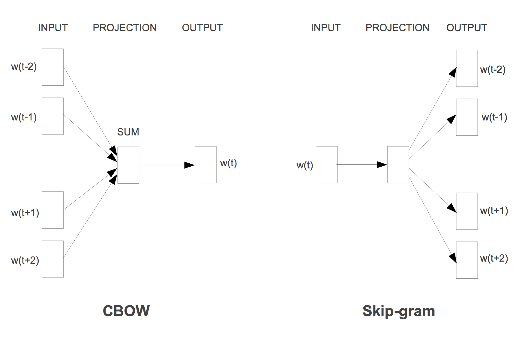
Continuous Bag-of-Words Model (CBOW)

• Similar to feedforward NNLM, but the non-linear hidden layer is removed.

• Projection layer is shared for all the words. So all words are projected into the same position and their vectors are averaged.

• Model is called bag-of-words model because the order of words in the history or future does not influence the projections.

• Unlike NNLM, words from future are used to with the best result found with 4 history and 4 future words in context.

• Training criterion is the correct classification of the current(middle) word.

• Training complexity is given by

\[Q = N * D + D * log_2(V)\]

• Model is continuous bag-of-words because unlike standard bag-of-words it uses continuous distributed representations of the context.

• Weights between the input and the projection layer is shared for all words positions in the same way as in NNLM.

Continuous Skip-Gram Model

• Similar to CBOW but slight changes in training criterion.

• Instead of predicting current word from the surrounding words in the window, current word is used to predict the words surrounding the current word.

• Accuracy and quality of vector is found to increase as the number of context words predicted is increased, but that increased the computational complexity as well.

• Training complexity is given by

\[Q = C * (D + D * log_2(V))\]

• Where
  • C is the maximum distance of the words. Say, C=5 is chosen then a number \(R \in [1, C]\) is selected randomly and then R words from history and R from future are correct labels of the current word.

Model Architectures

Results

• Algebraic operations on the vector representations actually give meaningful results like cosine similary of \(vector(X)\) is closest to \(vector(‘smallest’)\) where

\[vector(X) = vector(‘biggest’) - vector(‘big’) + vector(‘small’)\]

• Subtle relationships are learnt when accurate data is used. For example, France is to Paris as Germany is to Berlin.

• After a certain point adding more dimensionality to the word vectors or adding more training data provides diminishing improvements.

• NNLM vectors work better than RNNLM because word vectors in RNNLM are directly connected to non-linear hidden layer.

• CBOW is better than NNLM on syntactic tasks and about the same on semantic tasks.

• Skip-Gram works slightly worse than CBOW but better than NNLM on syntactic tasks and much better on semantic tasks.

• Training time for Skip-Gram model is greater than CBOW model.

REFERENCES:

Efficient Estimation of Word Representations in Vector Space