Basics of Machine Learning Series
Linear Regression
Linear regression is an approach for modeling the relationship between a scalar dependent variable y and one or more explanatory variables (or independent variables) denoted X. The case of one explanatory variable is called simple linear regression or univariate linear regression. For more than one explanatory variable, the process is called multiple linear regression. In linear regression, the relationships are modeled using linear predictor functions whose unknown model parameters are estimated from the data. Such models are called linear models.
Hypothesis
The hypothesis for a univariate linear regression model is given by,
- Where
- \(h_\theta (x)\) is the hypothesis function, also denoted as \(h(x)\) sometimes
- \(x\) is the independent variable
- \(\theta_0\) and \(\theta_1\) are the parameters of the linear regression that need to be learnt
Parameters of the Hypothesis
In the above case of the hypothesis, \(\theta_0\) and \(\theta_1\) are the parameters of the hypothesis. In case of a univariate linear regression, \(\theta_0\) is the y-intercept and \(\theta_1\) is the slope of the line.
Different values for these parameters will give different hypothesis function based on the values of slope and intercepts.
Cost Function of Linear Regression
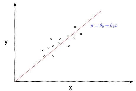
Assume we are given a dataset as plotted by the ‘x’ marks in the plot above. The aim of the linear regression is to find a line similar to the blue line in the plot above that fits the given set of training example best. Internally this line is a result of the parameters \(\theta_0\) and \(\theta_1\). So the objective of the learning algorithm is to find the best parameters to fit the dataset i.e. choose \(\theta_0\) and \(\theta_1\) so that \(h_\theta (x)\) is close to y for the training examples (x, y). This can be mathematically represented as,
- Where
- \(h_\theta(x^{(i)}) = \theta_0 + \theta_1\,x^{(i)} \)
- \((x^{(i)},y^{(i)})\) is the \(i^{th}\) training data
- m is the number of training example
- \({1 \over 2}\) is a constant that helps cancel 2 in derivative of the function when doing calculations for gradient descent
So, cost function is defined as follows,
which is basically \( {1 \over 2} \bar{x}\) where \(\bar{x}\) is the mean of squares of \(h_\theta(x^{(i)}) - y^{(i)}\), or the difference between the predicted value and the actual value.
And learning objective is to minimize the cost function i.e.
This cost function is also called the squared error function because of obvious reasons. It is the most commonly used cost function for linear regression as it is simple and performs well.
Understanding Cost Function
Cost function and Hypthesis are two different concepts and are often mixed up. Some of the key differences to remember are,
| Hypothesis \(h_\theta(x)\) | Cost Function \(J(\theta_1)\) |
|---|---|
| For a fixed value of \(\theta_1\), function of x | Function of parameter \(\theta_1\) |
| Each value of \(\theta_1\) corresponds to a different hypothesis as it is the slope of the line | For any such value of \(\theta_1\), \(J(\theta_1)\) can be calculated using (3) by setting \(\theta_0 = 0\) |
| It is a linear line or a hyperplane | Squared error cost function given in (3) is convex in nature |
Consider a simple case of hypothesis by setting \(\theta_0 = 0\), then (1) becomes
which corresponds to different lines passing through the origin as shown in plots below as y-intercept i.e. \(\theta_0\) is nulled out.
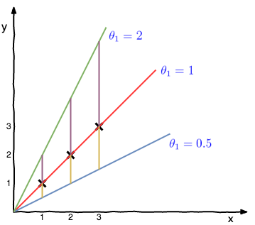
For the given training data, i.e. x’s marked on the graph, one can calculate cost function at different values of \(\theta_1\) using (3) which can be expressed in the following form using (5),
At \(\theta_1 = 2\),
At \(\theta_1 = 1\),
At \(\theta_1 = 0.5\),
On plotting points like this further, one gets the following graph for the cost function which is dependent on parameter \(\theta_1\).
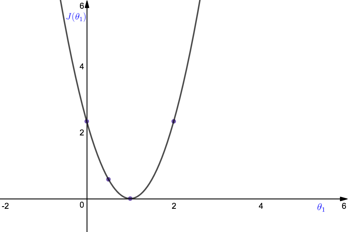
In the above plot each value of \(\theta_1\) corresponds to a different hypothesis. The optimization objective was to minimize the value of \(J(\theta_1)\) from (4), and it can be seen that the hypothesis correponding to the minimum \(J(\theta_1)\) would be the best fitting straight line through the dataset.
The issue lies in the fact that we cannot always find the optimum global minima of the plot manually because as the number of dimensions increase, these plots would be much more difficult to visualize and interpret. So there is a need of an automated algorithm that can help achieve this objective.
REFERENCES:
Machine Learning: Coursera - Cost Function
Machine Learning: Coursera - Cost Function Intuition I
Linear Regression: Wikipedia - Cost Function