Basics of Machine Learning Series

Index

Gradient Descent

Gradient descent is a first-order iterative optimization algorithm for finding the minimum of a function. To find a local minimum of a function using gradient descent, one takes steps proportional to the negative of the gradient (or of the approximate gradient) of the function at the current point. If instead one takes steps proportional to the positive of the gradient, one approaches a local maximum of that function; the procedure is then known as gradient ascent. Gradient descent is also known as steepest descent.

What and How ?

In the post Cost Function of Linear Regression, it was deduced that in order to find the best hypothesis, it is required to minimize the cost fuction \(J(\theta_0, \theta_1)\). And it is not always possible to achieve this goal manually as the complexity and dimensionality of the problem increases.

To summarize, given the cost function \(J(\theta_0, \theta_1)\), the objective is,

This is where gradient descent steps in. There are two basic steps involved in this algorithm:

• Start with some random value of \(\theta_0\), \(\theta_1\).

• Keep updating the value of \(\theta_0\), \(\theta_1\) to reduce \(J(\theta_0, \theta_1)\) until minimum is reached.

Actually graident descent is a much more robust algorithm capable of solving higher dimensionality problems as well i.e. given a cost fuction \(J(\theta_0, \theta_1, … , \theta_n)\), it can help achieve,

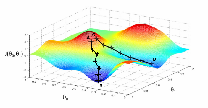
Depending on initialization gradient descent can end up in different local minimas and a unique solution is not guaranteed. It can be seen in the plot above, if the initialization is at point A then it leads to B while if the initialization is at point C then it would lead to point D after execution.

Definition

• Where
  • := is the assignment operator
  • \(\alpha\) is the learning rate which basically defines how big the steps are during the descent
  • \( \frac {\partial} {\partial \theta_j} J(\theta_0, \theta_1)\) is the partial derivative term
  • j = 0, 1 represents the feature index number

Also the parameters should be updated simulatenously, i.e. ,

The notion of simulatenous update is introduced because that is how the gradient descent would work naturally i.e. in nature the path taken at a point would be defined by the gradient along components at a point. But if the update is not simulatenous then the gradient is not computed at the same point because the updated value of one parameter is used in calculating the update of another. In practice this method might also work without any issues or behave strangely in some other cases, so by definition and the intuition of the gradient descent it would be incorrect implementation and would represent some other algorithm with properties different from those of gradient descent.

Understanding Gradient Descent

Consider a simpler cost function \(J(\theta_1)\) and the objective,

As defined earlier, start off by random initialization say at point A as shown in the plot below. Then according to the update definition of the algorithm, the derivative term is represented by the slope at any point also shown in the plot. In this case it would be a positive slope and since \(\alpha\) is a positive real number the overall term \(- \alpha \frac {d} {d \theta_1} J(\theta_1)\) would be negative. This means the value of \(\theta_1\) will be decreased in magnitude as shown by the arrows.

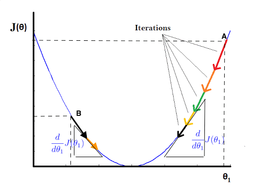
Similary, if the initialization was at point B, then the slope of the line would be negative and then update term would be positive leading to increase in the value of \(\theta_1\) as shown in the plot. So, no matter where the \(\theta_1\) is initialized, the algorithm ensures that parameter is updated in the right direction towards the minima, given proper value for \(\alpha\) is chosen.

This is intuitive because that is exactly what is needed for minimizing the cost function. The term \(alpha\), as it can be seen from the equation will determine the magnitude of the update term, \(- \alpha \frac {d} {d \theta_1} J(\theta_1)\) i.e. if the value is higher the steps of update would be proportionally larger.

Learning Rate, \(\alpha\)

A proper value of \(\alpha\) plays an important role in gradient descent. Choose an alpha too small and the algorithm will converge very slowly or get stuck in the local minima. Choose an \(\alpha\) too big and the algorithm will never converge either because it will oscillate between around the minima or it will diverge by overshooting the range. All these cases can be adequately understood by the plots below.

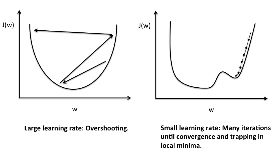
The plot on the left shows a large learning rate. This leads to overshooting because the steps taken by the algorithm in updating the parameters are so big that the optimization problem can never converge to the minima. Instead it overshoots with every iteration to either start diverging or to oscillate between points that are not the optimum solution.

The plot on the right is the case where learning rate is too small. As a result the steps taken i.e. the updates to the parameter \(\theta_n\) are so small that it would take a very long time to converge. More so because as we approach the minima the value of the slope i.e. the value of the differential term will also decrease and as a result the update term i.e. the product of small \(\alpha\) and small differential term would effect only a minute change. The other issue associated with the small learning rate is that of getting stuck in a local minima and hence never reaching the global minima.

Gradient descent can converge to a local optimum, even with a fixed learning rate. Because as we approach the local minimum, gradient descent will automatically take smaller steps as the value of slope i.e. derivative decreases around the local minimum.

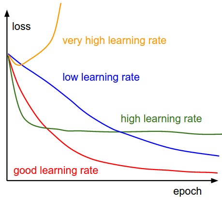
The plot above tries to summarize the effect of \(\alpha\) value on the convergence of the graident descent algorithm.

• The yellow plot shows the divergence of the algorithm when the learning rate is really high wherein the learning steps overshoot.
• The green plot shows the case where learning rate is not as large as the previous case but is high enough that the steps keep oscillating at a point which is not the minima.
• The red plot would be the optimum curve for the cost drop as it drops steeply initially and then saturates very close to the optimum value.
• The blue plot is the least value of \(\alpha\) and converges very slowly as the steps taken by the algorithm during update steps are very small.

Summary

Gradient Descent is an optimization algorithm. It can be applied to minimize any cost function J, and not just to linear regression. It is a rather generalized powerful technique widely used in learning problems to reach the optimum parameter sets. It is coupled with various learning techniques and works perfectly well with all of them. For example gradient descent works equally well with linear regression and neural networks.

REFERENCES:

Machine Learning: Coursera - Gradient Descent