Basics of Machine Learning Series
Introduction
The posts Cost Function of Linear Regression and Gradient Descent introduced the linear regression cost function and the gradient descent algorithm individually. If the gradient descent is applied to the linear regression cost function would help reach an optimal solution without much manual intervention.
Gradient Descent
Gradient descent algorithm can be summarized as,
- Where
- := is the assignment operator
- \(\alpha\) is the learning rate which basically defines how big the steps are during the descent
- \( \frac {\partial} {\partial \theta_j} J(\theta_0, \theta_1)\) is the partial derivative term
- j = 0, 1 represents the feature index number
Linear Regression
Linear regression hypothesis is given by,
And the corresponding cost function is given by,
Gradient Descent for Linear Regression
Gradient descent is applied to the optimazation problem of the cost function of the linear regression given in (2) in order to find parameters that minimize the cost.
In order to apply gradient descent, the derivative term i.e. \(\frac {\partial} {\partial \theta_j} J(\theta_0, \theta_1)\) needs to be calculated.
Updating the values of the derivative term in the gradient descent algorithm given in (1) where the update must be done simultaneously,
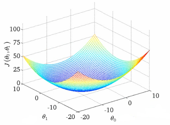
The cost function for a linear regression is a convex function i.e. a bow-shaped function and has only one global minimum and no local minima. So it does not face the issue of getting stuck in local minima. It can be understood better with the below plots.
The gradient descent technique that uses all the training examples in each step is called Batch Gradient Descent. This is basically the calculation of the derivative term over all the training examples as it can be seen it the equation above.
The equation of linear regression can also be solved using Normal Equations method, but it poses a disadvantage that it does not scale very well on larger data while gradient descent does.
Implementation
import random
import matplotlib.pyplot as plt
import math
import numpy as np

"""
Dummy Data for Linear Regression
"""
data = [(1, 1), (2, 2), (3, 4), (4, 3), (5, 5.5), (6, 8), (7, 6), (8, 8.4), (9, 10), (5, 4)]

"""
Plot the line using theta_values
"""
def plot_line(formula, x_range):
    x = np.array(x_range)
    y = formula(x)
    plt.plot(x, y)

"""
Hypothesis Function
"""
def h(x, theta_0, theta_1):
    return theta_0 + theta_1 * x

"""
Partial Derivative w.r.t. theta_1
"""
def j_prime_theta_1(data, theta_0, theta_1):
    result = 0
    m = len(data)
    for x, y in data :
        result += (h(x, theta_0, theta_1) - y) * x

    return (1/m) * result

"""
Partial Derivative w.r.t. theta_0
"""
def j_prime_theta_0(data, theta_0, theta_1):
    result = 0
    m = len(data)
    for x, y in data :
        result += (h(x, theta_0, theta_1) - y)
    return (1/m) * result

"""
Cost Function
"""
def j(data, theta_0, theta_1):
    cost = 0
    m = len(data)
    for x, y in data:
        cost += math.pow(h(x, theta_0, theta_1) - y, 2)
    return (1/(2*m)) * cost

"""
Simultaneous Update
"""
def update_theta(data, alpha, theta_0, theta_1):
    temp_0 = theta_0 - alpha * j_prime_theta_0(data, theta_0, theta_1)
    temp_1 = theta_1 - alpha * j_prime_theta_1(data, theta_0, theta_1)
    theta_0 = temp_0
    theta_1 = temp_1
    return theta_0, theta_1

"""
Gradient Descent For Linear Regression
"""
def gradient_descent(data, alpha, tolerance, theta_0=None, theta_1=None):
    if not theta_0:
        theta_0 = random.random() * 100
    if not theta_1:
        theta_1 = random.random() * 100
    prev_j = 10000
    curr_j = j(data, theta_0, theta_1)
    theta_0_history = []
    theta_1_history = []
    cost_history = []
    while(abs(curr_j - prev_j) > tolerance):
        try:
            cost_history.append(curr_j)
            theta_0_history.append(theta_0)
            theta_1_history.append(theta_1)
            theta_0, theta_1 = update_theta(data, alpha, theta_0, theta_1)
            prev_j = curr_j
            curr_j = j(data, theta_0, theta_1)
        except:
            break
    print("Stopped with Error at %.5f" % prev_j)
    return theta_0, theta_1

theta_0, theta_1 = gradient_descent(data, alpha=0.01, tolerance=0.00001)
The plot shows the adjustment of the values of \(\theta_0\) and \(\theta_1\) for fitting the best line through the given data points.
REFERENCES:
Machine Learning: Coursera - Gradient Descent for Linear Regression