Multivariate Linear Regression

When linear regression is applied on a higher-dimensional dataset, a generalization of linear regression is obtained

· · ·

Basics of Machine Learning Series

Index

· · ·

Introduction

Multivariate linear regression is the generalization of the univariate linear regression seen earlier i.e. Cost Function of Linear Regression. As the name suggests, there are more than one independent variables, $x_1, x_2 \cdots, x_n$ and a dependent variable $y$.

Notation

$x_1, x_2 \cdots, x_n$ denote the n features
$y$ denotes the output variable to be predicted
$n$ is number of features
$m$ is the number of training examples
$x^{(i)}$ is the $i^{th}$ training example
$x_j^{(i)}$ is the $j^{th}$ feature of the $i^{th}$ training example

Hypothesis

The hypothesis in case of univariate linear regression was,

$h_\theta(x) = \theta_0 + \theta_1\,x$

Extending the above function to multiple features, hypothesis of multivariate linear regression is given by,

$\begin{align} h_\theta(x) &= \theta_0 + \theta_1\,x_1 + \theta_2\,x_2 + \cdots + \theta_n\,x_n \\ &= \theta_0\,x_0 + \theta_1\,x_1 + \theta_2\,x_2 + \cdots + \theta_n\,x_n \text{, where }x_0 = 1 \\ &= \theta^T x \text{, vectorizing above equation} \end{align} \tag{1}$

Where,
- $\theta = \begin{bmatrix} \theta_0 \\ \theta_1 \\ \vdots \\ \theta_n \\ \end{bmatrix} \in \mathbb{R}^{n+1}$ and $x = \begin{bmatrix} x_0 \\ x_1 \\ \vdots \\ x_n \\ \end{bmatrix} \in \mathbb{R}^{n+1} $

Cost Function

The cost function for univariate linear regression was,

$J(\theta_0, \theta_1) = {1 \over 2m} \sum_{i=1}^m \left( h_\theta(x^{(i)}) - y^{(i)} \right)^2$

Extending the above function to multiple features, the cost function for multiple features is given by,

$\begin{align} J(\theta) &= {1 \over 2m} \sum_{i=1}^m \left( h_\theta(x^{(i)}) - y^{(i)} \right)^2 \\ &= {1 \over 2m} \sum_{i=1}^m \left( \theta^T x^{(i)} - y^{(i)} \right)^2 \\ &= {1 \over 2m} \sum_{i=1}^m \left( \left( \sum_{j=0}^n \theta_j x_j^{(i)} \right) - y^{(i)} \right)^2 \\ \end{align} \tag{2}$

Where $\theta$ is a vector give by $\theta = \begin{bmatrix} \theta_0 \\ \theta_1 \\ \vdots \\ \theta_n \\ \end{bmatrix} $

Gradient Descent

$\begin{align} \text{repeat until convergence} \begin{cases} \theta_j := \theta_j - \alpha {\partial \over \partial \theta_j} J(\theta) \\ \end{cases} \end{align} \tag{3}$

Note: simultaneous update only

Evaluating the partial derivative ${\partial \over \partial \theta_j} J(\theta)$ gives,

${\partial \over \partial \theta_j} J(\theta) = {1 \over m} \sum_{i=1}^m \left( h_\theta(x^{(i)}) - y^{(i)} \right) x_j^{(i)} \tag{4}$

It can be easily seen that (4) is generalization of the update equation for univariate linear regression, because if we take only two features $\theta_0$ and $\theta_1$ and substitute in (4) the values, it results in the same equations as in Univariate Linear Regression

Feature Scaling

It is found that during gradient descent if the features are on the same scale then the algorithm tends to work better than when the features are not appropriately scaled in the same range.

The plot below shows the effect of feature scaling on the contour plot of the cost function of hypothesis based on these features.

Feature Scaling and Contour Plot

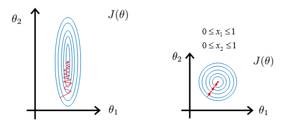
As seen above, if the contours are skewed then learning steps would take longer to converge as the steps would be more prone to oscillatory behaviour as shown in the left plot. Whereas if the features are properly scaled, then the plot is evenly distributed and the steps of gradient descent have better profile of convergence.

Scaling of features between 0 and 1 is achieved by dividing the features by max. This helps in keeping all the features in appropriate ranges. The aim is to ideally keep the features around the range -1 to 1.

Different ways of achieving feature scaling:

Normalization: Divide each feature by max of the feature column.
Mean Normalization: Replace a feature $x_i$ with $x_i - \mu_i$ so that the approximate mean of the features is 0 which is then normalized. Not applied to the feature $x_0$

$x_i = \frac {x_i - \mu_i} {S_i} \forall i \in \{1, 2, \cdots, n\}$

Where
- $x_i$ is the feature value
- $\mu_i$ is the mean
- $S_i$ is the standard deviation or the range i.e. $max - min$

Learning Rate

There are several ways of debugging the gradient descent algorithm. One of the ways is to plot the graph of cost function as a function of number of epochs. If the value is decreasing for every epoch then the descent is working fine.

Learning Rate

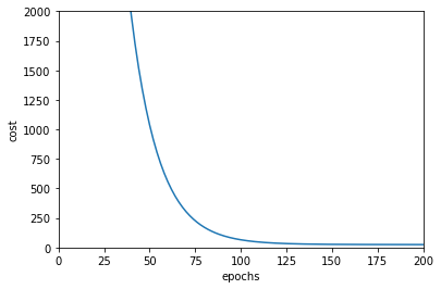
If the curve is plotted as shown one can easily infer that a saturation is reached after 150 iterations.

Automatic Convergence Test: Gradient descent can be considered to be converged if the drop in cost function is not more than a preset threshold say $10^{-3}$

Looking at the plot can point out if the algorithm is not working properly.

Learning Rate

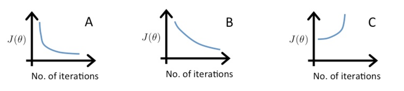
For example, plot A is a proper learning curve but if the plot shows that value of cost function is increasing as in plot C, then this indicates the algorithm is diverging. It generally happens if the value of learning rate $\alpha$ is too high.

Also, if the plot shows that the value is oscillating or fluctuating then the learning rate needs to be reduced as the steps are not small enough to proceed to the minima.

For sufficiently small $\alpha$, gradient descent should decrease on every iteration.

Very small learning rate is not advisable as the algorithm will be slow to converge as seen in plot B.

In order to choose optimum value of $\alpha$ run the algorithm with different values like, 1, 0.3, 0.1, 0.03, 0.01 etc and plot the learning curve to understand whether the value should be increased or descreased.

Feature Engineering

Sometimes it might be fruitful to generate new features by combining the existing ones. For example, given width and length of a property to predict price it might be helpful to use area of the property i.e. width * length as an additional feature.

Polynomial Regression

The concept of feature engineering can be used to achieve polynomial regression. Say the polynomial hypothesis chosen is,

$h_\theta(x) = \theta_0 + \theta_1\,x + \theta_2\,x^2 + \cdots + \theta^n\,x^n$

This function can be addressed as multivariate linear regression by substitution and is given by,

$h_\theta(x) = \theta_0 + \theta_1\,x_1 + \theta_2\,x_2 + \cdots + \theta_n\,x_n$

Where $x_n = x^n$

Note: if using features like this then it is very important to apply feature scaling in order to avert issues related to feature range imbalance.

This technique can be very powerful because one can fit all types of features using the substitution model. For example one can get a non-decreasing function as opposed to quadratic function which comes back down by using the following function

$h_\theta(x) = \theta_0 + \theta_1\,x + \theta_2\,\sqrt{x}$

Implementation

import random
import matplotlib.pyplot as plt
import math
import numpy as np

"""
Dummy Data for Multivariate Regression
"""
data = [(1, 1), (2, 2), (3, 4), (4, 3), (5, 5.5), (6, 8), (7, 6), (8, 8.4), (9, 10), (5, 4)]    

"""
Plot the line using theta_values
"""
def plot_line(formula, x_range, order_of_regression):
    x = np.array(x_range).tolist()  
    y = [formula(update_features(x_i, order_of_regression)) for x_i in x]
    plt.plot(x, y)

"""
Hypothesis Function
"""
def h(x, theta):
    return np.matmul(theta.T, x)[0][0]

"""
Partial Derivative w.r.t. theta_i
"""
def j_prime_theta(data, theta, order_of_regression, i):
    result = 0
    m = len(data)
    for x, y in data :
        x = update_features(x, order_of_regression)
        result += (h(x, theta) - y) * x[i]
    
    return (1/m) * result

"""
Update features by order of the regression
"""

def update_features(x, order_of_regression):
    features = [1]
    for i in range(order_of_regression):
        features.append(math.pow(x, i+1))
    return np.atleast_2d(features).T

"""
Cost Function
"""
def j(data, theta, order_of_regression):
    cost = 0
    m = len(data)
    for x, y in data:
        x = update_features(x, order_of_regression)
        cost += math.pow(h(x, theta) - y, 2)
    return (1/(2*m)) * cost

"""
Simultaneous Update
"""
def update_theta(data, alpha, theta, order_of_regression):
    temp = []
    for i in range(order_of_regression+1):
        temp.append(theta[i] - alpha * j_prime_theta(data, theta, order_of_regression, i))
    theta = np.array(temp)
    return theta
    
"""
Gradient Descent For Multivariate Regression
"""
def gradient_descent(data, alpha, tolerance, theta=[], order_of_regression = 2):
    if len(theta) == 0:
        theta = np.atleast_2d(np.random.random(order_of_regression+1) * 100).T
    prev_j = 10000
    curr_j = j(data, theta, order_of_regression)
    print(curr_j)
    cost_history = []
    theta_history = [] 
    while(abs(curr_j - prev_j) > tolerance):
        try:
            cost_history.append(curr_j)
            theta_history.append(theta)
            theta = update_theta(data, alpha, theta, order_of_regression)
            prev_j = curr_j
            curr_j = j(data, theta, order_of_regression)
            print(curr_j)
        except:
            break
    print("Stopped with Error at %.5f" % prev_j)
    return theta

theta = gradient_descent(data, 0.001, 0.001)

Multivariate Regression

The above plot shows the working of multivariate linear regression to fit polynomial curve. The higher order terms of the polynomial hypothesis are fed as separate features in the regression. The plot is the shape of a parabola which is consistent with the shape of curves of second order polynomials.

Note: The implementation above does not have scaled features. It would be harder to make the algorithm converge if the features are not scaled. But if they are scaled properly, not only does the algorithm converges better but also faster. Below is the plot of the curve fitting by gradient descent when the features are scaled appropriately.

Multivariate Regression

A rough implementation of the feature scaling used to get the plot above can be found here.

REFERENCES:

Machine Learning: Coursera - Multivariate Linear Regression
Machine Learning: Coursera - Gradient Descent for Multiple Variables
Machine Learning: Coursera - Gradient Descent in Practice I - Feature Scaling
Machine Learning: Coursera - Gradient Descent in Practice II - Learning Rate
Machine Learning: Coursera - Feature and Polynomial Regerssion

· · ·

Shams S

AIML Resident @ Apple

Multivariate Linear Regression

When linear regression is applied on a higher-dimensional dataset, a generalization of linear regression is obtained

Basics of Machine Learning Series

Introduction

Notation

Hypothesis

Cost Function

Gradient Descent

Feature Scaling

Learning Rate

Feature Engineering

Polynomial Regression

Implementation

REFERENCES:

Notes

Recursing the Rabbit Hole