Normal Equation

Given a matrix equation, the normal equation is one which minimizes the sum of the square differences between the left and right sides

· · ·

Basics of Machine Learning Series

Index

· · ·

Introduction

Gradient descent is an algorithm which is used to reach an optimal solution iteratively using the gradient of the loss function or the cost function. In contrast, normal equation is a method that helps solve for the parameters analytically i.e. instead of reaching the solution iteratively, solution for the parameter $\theta$ is reached at directly by solving the normal equation.

Intuition

Consider a one-dimensional equation for the cost function given by,

$J(\theta) = a\theta^2 + b\theta + c \tag{1}$

Where $\theta \in \mathbb{R} $

According to calculus, one can find the minimum of this function by calculating the derivative and solving the equation by setting derivative equal to zero, i.e.

${d \over d\theta} J(\theta) = 0 \tag{2}$

Similarly, extending (1) to multi-dimensional setup, the cost function is given by,

$J(\theta_0, \theta_1, \cdots, \theta_n) = {1 \over 2m} \sum_{i=1}^m \left( h_\theta(x^{(i)}) - y^{(i)} \right)^2 \tag{3}$

Where
- $\theta \in \mathbb{R}^{n+1} $
- n is the number of features
- m is the number of training samples

And similar to (2), the minimum of (3) can be found by taking partial derivatives w.r.t. individual $\theta_i \forall i \in (0, 1, 2, \cdots, n) $ and solving the equations by setting them to zero, i.e.

${\partial \over \partial \theta_i}J(\theta) = 0 \tag{4}$

where $i \in (0, 1, 2, \cdots, n)$

Through derivation one can find that $\theta$ is given by,

$\theta = \left( X^TX \right)^{-1}X^Ty \tag{5}$

Feature scaling is not necessary for the normal equation method. Reason being, the feature scaling was implemented to prevent any skewness in the contour plot of the cost function which affects the gradient descent but the analytical solution using normal equation does not suffer from the same drawback.

Comparison between Gradient Descent and Normal Equation

Given m training examples, and n features

Gradient Descent	Normal Equation
Proper choice of $\alpha$ is important	$\alpha$ is not needed
Iterative Method	Direct Solution
Works well with large n. Complexity of algorithm is O($kn^2$)	Slow for large n. Need to compute $(X^TX)^{-1}$. Generally the cost for computing the inverse is O($n^3$)

Generally if the number of features is less than 10000, one can use normal equation to get the solution beyond which the order of growth of the algorithm will make the computation very slow.

Non-invertibility

Matrices that do not have an inverse are called singular or degenerate.

Reasons for non-invertibility:

Linearly dependent features i.e. redundant features.
Too many features i.e. $m \leq n$, then reduce the number of features or use regularization.

Calculating psuedo-inverse instead of inverse can also solve the issue of non-invertibility.

Implementation

import matplotlib.pyplot as plt
import numpy as np

"""
Dummy Data for Linear Regression
"""
data = [(1, 1), (2, 2), (3, 4), (4, 3), (5, 5.5), (6, 8), (7, 6), (8, 8.4), (9, 10), (5, 4)]    

"""
Matrix Operations
"""
inv = np.linalg.inv
mul = np.matmul

X = []
y = []
for x_i, y_i in data:
    X.append([1, x_i])
    y.append(y_i)
X = np.array(X)
y = np.atleast_2d(y).T

"""
Theta Calculation Using equation (5)
"""
theta = mul(mul(inv(mul(X.T, X)), X.T), y)

"""
Prediction of y using theta
"""
y_pred = np.matmul(X, theta)

"""
Plot Graph
"""
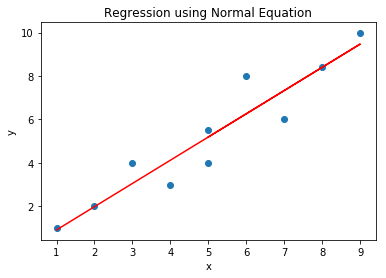
plt.scatter([i[0] for i in data], [i[1] for i in data])
plt.plot([i[0] for i in data], y_pred, 'r')
plt.title('Regression using Normal Equation')
plt.xlabel('x')
plt.ylabel('y')
plt.show()

Normal Equation Solution

Derivation of Normal Equation

Given the hypothesis,

$\begin{align} h_\theta(x) &= \theta_0\,x_0 + \theta_1\,x_1 + \cdots + \theta_n\,x_n \\ &= \theta_T\,x \\ \end{align} \tag{6}$

$\theta = \begin{bmatrix} \theta_0 \\ \theta_1 \\ \vdots \\ \theta_n \end{bmatrix} $

Let X be the design matrix wherein each row corresponds to the features in $i^{th}$ sample of the m samples. Similarly, y is the vector with all the target values for all the m training samples. The cost function for the hypothesis (6) is given by (3). The cost function can be vectorized as follows for replacing the sigma operation with the sum over terms for matrix multiplication,

$\begin{align} J(\theta) &= {1 \over 2m} \left( X\theta - y \right)^T \left( X\theta - y \right) \\ & = {1 \over 2m} \left( (X\theta)^T - y^T \right) \left( X\theta - y \right) \\ & = {1 \over 2m} \left( (X\theta)^TX\theta - (X\theta)^Ty - y^T(X\theta) + y^Ty \right) \\ \end{align} \tag{7}$

Since $X\theta$ and $y$ both are vectors, $(X\theta)^Ty = y^T(X\theta)$. So (7) can be further simplified as,

$J(\theta) = {1 \over 2m} \left( (X\theta)^TX\theta - 2(X\theta)^Ty + y^Ty \right)$

Taking partial derivative w.r.t $\theta$ and equating to zero,

${\partial \over \partial \theta} \left( (X\theta)^TX\theta - 2(X\theta)^Ty \right) = 0 \tag{8}$

Let,

$\begin{align} Q(\theta) &= 2(X\theta)^Ty \\ &= 2 \theta^T X^T y \\ &= 2 \begin{bmatrix} \theta_0 & \cdots & \theta_n \end{bmatrix} \begin{bmatrix} x_{10} & \cdots & x_{m0} \\ x_{11} & \cdots & x_{m1} \\ \vdots & \ddots & \vdots \\ x_{1n} & \cdots & x_{mn} \\ \end{bmatrix} \begin{bmatrix} y_{1} \\ \vdots \\ y_{m} \end{bmatrix}\\ &= 2 \begin{bmatrix} (\theta_0 * x_{10} + \cdots + \theta_n * x_{1n}) \cdots (\theta_0 * x_{m0} + \cdots + \theta_n * x_{mn}) \\ \end{bmatrix} \begin{bmatrix} y_{1} \\ \vdots \\ y_{m} \end{bmatrix}\\ &= 2 \begin{bmatrix} (\theta_0 * x_{10} + \cdots + \theta_n * x_{1n})y_1 \cdots (\theta_0 * x_{m0} + \cdots + \theta_n * x_{mn})y_m \\ \end{bmatrix} \\ &= 2 \sum_{i=1}^m y_i \sum_{j=0}^n \theta_j * x_{ij} \end{align} \tag{9}$

Taking partial derivatives,

$\begin{align} {\partial Q \over \partial \theta_0} &= 2(x_{10}y_1 + \cdots + x_{m0}y_m) \\ & \vdots \\ {\partial Q \over \partial \theta_n} &= 2(x_{1n}y_1 + \cdots + x_{mn}y_m) \\ \end{align} \tag{10}$

Vectorizing (10),

${\partial Q \over \partial \theta} = 2X^Ty \tag{11}$

Similarly, let,

$\begin{align} P(\theta)&= (X\theta)^T(X\theta) \\ &= \theta^T X^T X \theta \\ &= \begin{bmatrix} \theta_0 \cdots \theta_n \end{bmatrix} \begin{bmatrix} x_{10} & \cdots & x_{m0} \\ x_{11} & \cdots & x_{m1} \\ \vdots & \ddots & \vdots \\ x_{1n} & \cdots & x_{mn} \end{bmatrix} \begin{bmatrix} x_{10} & \cdots & x_{1n} \\ \vdots & \ddots & \vdots \\ x_{m0} & \cdots & x_{mn} \end{bmatrix} \begin{bmatrix} \theta_0 \\ \vdots \\ \theta_n \end{bmatrix} \\ &= \begin{bmatrix} (\theta_0x_{10} + \cdots + \theta_nx_{1n}) \cdots (\theta_0x_{m0} + \cdots + \theta_nx_{mn}) \end{bmatrix} \begin{bmatrix} (\theta_0x_{10} + \cdots + \theta_nx_{1n}) \\ \vdots \\ (\theta_0x_{m0} + \cdots + \theta_nx_{mn}) \end{bmatrix} \\ & = (\theta_0x_{10} + \cdots + \theta_nx_{1n})^2 + \cdots + (\theta_0x_{m0} + \cdots + \theta_nx_{mn})^2 \end{align}$

Taking partial derivatives,

$\begin{align} {\partial P \over \partial \theta_0} &= 2x_{10}(\theta_0x_{10} + \cdots + \theta_nx_{1n}) + \cdots + 2x_{m0}(\theta_0x_{m0} + \cdots + \theta_nx_{mn})\\ & \vdots \\ {\partial P \over \partial \theta_n} &= 2x_{1n}(\theta_0x_{10} + \cdots + \theta_nx_{1n}) + \cdots + 2x_{mn}(\theta_0x_{m0} + \cdots + \theta_nx_{mn}) \\ \end{align} \tag{12}$

Vectorizing above equations,

$\begin{align} {\partial P \over \partial \theta} &= 2 \begin{bmatrix} x_{10} & \cdots & x_{m0} \\ \vdots & \ddots & \vdots \\ x_{1n} & \cdots & x_{mn} \end{bmatrix} \begin{bmatrix} \theta_0x_{10} + \cdots + \theta_nx_{1n} \\ \vdots \\ \theta_0x_{m0} + \cdots + \theta_nx_{mn} \end{bmatrix} \\ &= 2 X^T \begin{bmatrix} x_{10} & \cdots & x_{1n} \\ \vdots & \ddots & \vdots \\ x_{m0} & \cdots & x_{mn} \end{bmatrix} \begin{bmatrix} \theta_0 \\ \vdots\\ \theta_n \end{bmatrix} \\ &= 2X^T X\theta \tag{13} \end{align}$

Substitution (13) and (11) in (8),

$2X^T X\theta = 2X^Ty$

If $X^T X$ is invertible, then,

$\theta = \left( X^TX \right)^{-1}X^Ty$

which is same as (5)

REFERENCES:

Machine Learning: Coursera - Normal Equation
Derivation of the Normal Equation for linear regression
Normal Equation and Matrix Calculus

· · ·

Shams S

AIML Resident @ Apple

Normal Equation

Given a matrix equation, the normal equation is one which minimizes the sum of the square differences between the left and right sides

Basics of Machine Learning Series

Introduction

Intuition

Comparison between Gradient Descent and Normal Equation

Non-invertibility

Implementation

Derivation of Normal Equation

REFERENCES:

Notes

Recursing the Rabbit Hole

Gradient Descent	Normal Equation
Proper choice of \(\alpha\) is important	\(\alpha\) is not needed
Iterative Method	Direct Solution
Works well with large n. Complexity of algorithm is O(\(kn^2\))	Slow for large n. Need to compute \((X^TX)^{-1}\). Generally the cost for computing the inverse is O(\(n^3\))