Basics of Machine Learning Series
Introduction
Classification is a supervised learning problem wherein the target variable is categorical unlike regression where the target variable is continuous. Classification can be binary i.e. only two possible values of the target variable or multi-class i.e. more than two categories.
The most basic step would be to try and fit regression curve to see if one can achieve classification using the same approach. Below is a plot attempting the same.
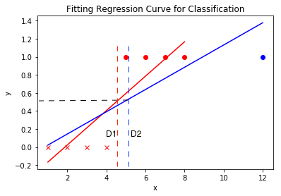
It can be seen below that the attempt to achieve classification using regression curve and thresholding will not always yield conclusive results. In first case say only red data points are in the dataset, then fitting the curve and setting the threshold at 0.5 would work, but say an outlier is present like the blue data point then the same decision boundary D1 would shift to D2 if the threshold is kept constant and the boundary would not be perfect. Hence there is a need of Decision Boundary instead of predictive curve.
Applying linear regression to classification problem might work in some cases but is not advisable as it would not scale with complexity.
Another issue with application of linear regession to classification would be that even know the categorical variables are discreet say 1s and 0s, the hypothesis would give continuous values which maybe much greater that 1 or much lesser than 0. This issue can be solved by using logistic regression where
Logistic Regression
Since (1) is to be true, the hypothesis from linear regression given by \(h_\theta(x) = \theta^T\,x\) will not work for logistic regression. Hence there is a need of squashing function i.e. a function which limits the output of hypothesis between given range. For logistic regression sigmoid function is used as the squashing function. The hypothesis for logistic regression is give by,
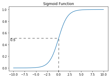
Where \(g(z) = {1 \over 1 + e^{-z}}\) and is called sigmoid function or logistic function. Plot of the sigmoid function is given below which shows no matter what the value of x, the function returns a value between 0 and 1 consistent with (1).
The value of hypothesis is interpretted as the probability that the input x belongs to class y=1. i.e. probability that y=1, given x, parametrized by \(\theta\).
It can be mathematically represented as,
The fundamental properties of probability holds here, i.e.,
Decision Boundary
for the given hypothesis of logistic regression in (2), say \(\delta=0.5\) is chosen as the threshold for the binary classification, i.e.
From the plot of sigmoid function, it is seen that
Using (6), (5) can be rewritten as,
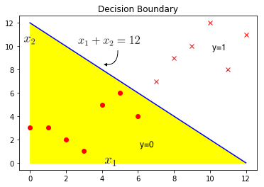
Suppose the training data is as show in the plot above where dots and Xs are the two different classes. Let the hypothesis \(h_\theta(x)\) and the optimal value of \(\theta\) be given by,
Using the \(\theta\) from (9) and hypothesis from (8) , (7) can be written as,
If the line \(x_1 + x_2 = 12\) is plotted as shown in the plot above then the region below i.e. the yellow region is where \(x_1 + x_2 \lt 12\) and predicted 0 and similarly the white region above the line \(x_1 + x_2 = 12\) is where \(x_1 + x_2 \geq 12\) and hence predicted 1. The line here is called the decision boundary. As the name suggests this line seperates the region with prediction 0 from region with prediction 1. Decision boundary and prediction regions are the property of the hypothesis and not of the dataset. Dataset is only used to fit the parameters, but once the parameters are determined they solely define the decision boundary
It is possible to achieve non-linear decision boundaries by using the higher order polynomial terms and can be encorporated in a way similar to how multivariate linear regression handles polynomial regression.
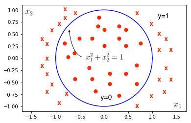
The plot above is an example of non-linear decision boundary using higher order polynomial logistic regression.
Say, the hypothesis of the logistic regression has higher order polynomial terms, and is given by,
The, \(\theta\) given below would form an apt decision boundary,
Substituting (12) in (11),
So, from (7), the decision boundary is given by,
Which the equation of a circle at origin with radius 0, as can be seen in the plot above. And, using the \(\theta\) from (12) and hypothesis from (11) , (7) can be written as,
As the order of features is increased more and more complex decision boundaries can be achieved by logistic regression.
Gradient Descent is used to fit the parameter values \(\theta\) in (9) and (12).
REFERENCES:
Machine Learning: Coursera - Classification
Machine Learning: Coursera - Hypothesis Representation
Machine Learning: Coursera - Decision Boundary