Logistic Regression Model

Mathematics and Implementation of training a logistic regression model

· · ·

Basics of Machine Learning Series

Index

· · ·

Introduction

Classifiction and Logistic Regression explains why logistic regression and intuition behind it. This post is about how the model works and some intuitions behind it.

Consider a training set having m examples,

$\{ (x^{(1)}, y^{(1)}),\, (x^{(2)}, y^{(2)}),\, \cdots ,\, (x^{(m)}, y^{(m)}) \}$

Where
- $x \in \begin{bmatrix} x_0 \\ x_1 \\ \vdots \\ x_m
  \end{bmatrix} \in \mathbb{R}^{n+1} $
- $x_0 = 1$
- $y \in {0, 1}$

And hypothesis is given by,

$h_\theta(x) = {1 \over 1 + e^{-\theta^Tx}} \tag{1}$

Cost Function

It can be seen in Mulivariate Linear Regression that the cost function for the linear regression is given by,

$\begin{align} J(\theta) &= {1 \over m} \sum_{i=1}^m {1 \over 2} \left( h_\theta(x^{(i)}) - y^{(i)} \right)^2 \\ &= {1 \over m} \sum_{i=1}^m Cost(h_\theta(x^{(i)}), y^{(i)}) \end{align} \tag{2}$

Where $Cost(h_\theta(x), y) $ is the cost the learning algorithm has to pay if it makes an error in the prediction and from (2), it is given by,

$Cost(h_\theta(x), y) = {1 \over 2} \left( h_\theta(x) - y \right)^2 \tag{3}$

In case of linear regression the value of cost depends on how off is the prediction of the regression from the expected value which works well for the optimization required in linear regression.

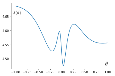
But this cost function would not work well for the logistic regression because the hypothesis for logistic regression is the complex sigmoid term shown in (1), gives non-convex curve with many local minima as shown in the plot below. So gradient descent will not work properly for such a case and therefore it would be very difficult to minimize this function.

Non Convex Cost

import math
import numpy as np
import matplotlib.pyplot as plt

x = np.array([-20, -5, -1,  10, -50, -10, 2, -3, 4, 1]).T
y = np.array([-1, 3, -2,  3, 4, -5, 1, 3, -4, 1]).T

mul = np.matmul

def j(x, y, theta):
    h = x*theta
    h = 1 / (1 + np.exp(-h))\
    d = h - y
    s = mul(d.T, d)
    return s/(len(x)*2)

theta = (np.array(range(-100, 100))/100).tolist()
cost = [j(x, y, i) for i in theta]
plt.plot(theta, cost)
plt.show()

So, cost function for logistic regression is given by,

$Cost(h_\theta(x), y) = \begin{cases} \begin{align} -log(h_\theta(x))\text{ if } y &= 1 \\ -log(1-h_\theta(x))\text{ if } y &= 0 \\ \end{align} \end{cases} \tag{4}$

The plots of the functions above can be seen below. It is clear that new cost function can be minimized because its convex.

Plot of Log Fucntions

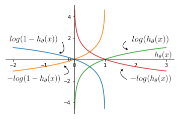
Other useful properties of the chosen cost function are:

if y = 1 and
- h(x) = 1, then Cost = 0
- h(x) $\to$ 0, then Cost $\to \infty$
if y = 0 and
- h(x) = 0, then Cost = 0
- h(x) $\to$ 1, then Cost $\to \infty$

Since $y \in \{0, 1\} $, (4) can be written as,

$Cost(h_\theta(x), y) = -y\,log(h_\theta(x) - (1-y)\,log(1 - h_\theta(x)) \tag{5}$

So, adding to (2),

$\begin{align} J(\theta) &= {1 \over m} \sum_{i=1}^m {1 \over 2} \left( h_\theta(x^{(i)}) - y^{(i)} \right)^2 \\ &= {1 \over m} \sum_{i=1}^m Cost(h_\theta(x^{(i)}), y^{(i)}) \\ &= -{1 \over m} \sum_{i=1}^m \left( y^{(i)}\,log(h_\theta(x^{(i)}) + (1-y^{(i)})\,log(1 - h_\theta(x^{(i)})) \right) \end{align} \tag{6}$

This cost function is reached at using the principle of maximum likelyhood expectation. So now to get optimal $\theta$,

$minimize_\theta J(\theta) \tag{7}$

Which is done using gradient descent given by,

$\begin{align} \text{repeat until convergence} \begin{cases} \theta_j := \theta_j - \alpha {\partial \over \partial \theta_j} J(\theta) \\ \end{cases} \end{align} \tag{7}$

And the differential term is given by,

$\begin{align} \frac {\partial} {\partial \theta} J(\theta) &= - \frac {\partial} {\partial \theta} {1 \over m} \sum_{i=1}^m \left( y^{(i)}\,log(h_\theta(x^{(i)})) + (1-y^{(i)})\,log(1 - h_\theta(x^{(i)})) \right) \\ &= - {1 \over m} \sum_{i=1}^m \left( y^{(i)}\, \frac {\partial} {\partial \theta}log(h_\theta(x^{(i)})) + (1-y^{(i)})\,\frac {\partial} {\partial \theta} log(1 - h_\theta(x^{(i)})) \right) \\ \end{align} \tag{8}$

Differential of log is given by,

${d \over dz} log(z) = {1 \over z} \tag{9}$

And differential of sigmoid function is given by,

$\begin{align} {d \over dz} h(z) &= {d \over dz} {1 \over 1 + e^{-z}} \\ &= {e^{-z} \over (1 + e^{-z})^2} \\ &= { 1 + e^{-z} - 1 \over (1 + e^{-z})^2} \\ &= { 1 \over 1 + e^{-z}} - {1 \over (1 + e^{-z})^2 } \\ &= h(z)(1-h(z)) \end{align} \tag{10}$

Using (9) and (10) in (8),

$\begin{align} {\partial \over \partial \theta_j} J(\theta) &= - {1 \over m} \sum_{i=1}^m y^{(i)}\, {x_j^{(i)} \over h(x^{(i)})} h(x^{(i)})(1-h(x^{(i)})) + (1-y^{(i)}) {x_j^{(i)} \over 1 - h(x^{(i)})} (-h(x^{(i)})(1-h(x^{(i)}))) \\ &= - {1 \over m} \sum_{i=1}^m ( y^{(i)}\,(1-h(x^{(i)})) - (1-y^{(i)}) h(x^{(i)}) ) x_j^{(i)} \\ &= - {1 \over m} \sum_{i=1}^m \left( y^{(i)} - y^{(i)} h(x^{(i)}) - h(x^{(i)}) + y^{(i)} h(x^{(i)}) \right) x_j^{(i)} \\ &= {1 \over m} \sum_{i=1}^m \left(h(x^{(i)}) - y^{(i)} \right) x_j^{(i)} \end{align} \tag{11}$

Using (11) in (7),

$\begin{align} \text{repeat until convergence} \begin{cases} \theta_j := \theta_j - \alpha {1 \over m} \sum_{i=1}^m \left(h(x^{(i)}) - y^{(i)} \right) x_j^{(i)} \end{cases} \end{align} \tag{12}$

Which looks same as the result of gradient descent of linear regression in Mulivariate Linear Regression. But there is a difference which can be seen in the defination of the hypothesis of linear regression and logistic regression.

Vectorizing (12),

$\theta := \theta - \alpha {1 \over m} \sum_{i=1}^m [(h_\theta(x^{(i)}) - y^{(i)}).x^{(i)}]$ $\theta := \theta - \alpha {1 \over m} X^T (g(X\theta) - y)$

Where X is the design matrix.

Note: Feature Scaling is as important for logistic regression as it is for linear regression as it helps the process of gradient descent.

Advanced Optimization

Given the functions for calculation of $J(\theta)$ and $\frac {\partial} {\partial \theta} J(\theta)$ one can apply one of the many optimization techniques other than gradient descent:

Conjugate Descent
BFGS
L-BFGS

Advantage	Disadvantages
No need to manually pick $\alpha$	More complex
Often faster than gradient descent	Harder to debug

Most of these algorithms have a clever inner loop like line search algorithm which automatically finds out the best $\alpha$ value.

Implementation

Below is an implementation for linear decision boundary,

import math
import numpy as np
import matplotlib.pyplot as plt
x = []
y = []
for _ in range(30):
    i = np.random.rand()
    x.append(i)
    y.append(round(i))
x.append(0)
y.append(1)
x = np.atleast_2d(x).T
y = np.atleast_2d(y).T
plt.scatter(x[np.where(y==1)], y[np.where(y==1)])
plt.scatter(x[np.where(y==0)], y[np.where(y==0)])

theta = np.random.randint(1, 100, size=(2, 1))/ 1000000
theta = np.array([[0.5], [0]])
mul = np.matmul
alpha = 0.6
m = len(x)
X = np.hstack((np.ones((len(x), 1)), x))

def h(X, theta):
    return 1 / (1 + np.exp(-mul(X, theta)))

def j(X, y, theta):
    return (-1/m) * (mul(y.T, np.log(h(X, theta))) + mul((1-y).T, np.log(1-h(X, theta))))

def update(X, y, theta):
    return theta - (alpha/m * mul(X.T, (h(X, theta) - y)))

prev_j = 10000
curr_j = j(X, y, theta)
tolerance = 0.000001
theta_history = [theta]
cost_history = [curr_j]

while(abs(curr_j - prev_j) > tolerance):
    theta = update(X, y, theta)
    theta_history.append(theta)
    prev_j = curr_j
    curr_j = j(X, y, theta)
    cost_history.append(curr_j[0][0])
print(curr_j[0][0])

plt.plot(x, mul(X, theta))
plt.show()

Linear Decision Boundary

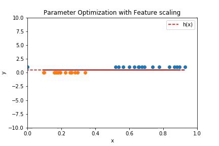
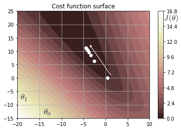
Plot above shows how the linear decision boundary fits the data over the iterations. The plot below is the contour plot of the cost function.

Contour Plot

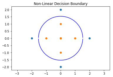
Following is an implementation of non-linear decision boundary. The code is similar to the previous implementation but the data and the dimensions of the design matrix vary because of higher number of features.

import math
import numpy as np
import matplotlib.pyplot as plt
x = np.array([
    [0,0], [0,1], [0, -1], [1, 0], [-1, 0],
    [0,2], [0, -2], [2, 0], [-2, 0]
])
y = np.atleast_2d([0, 0, 0, 0, 0, 1, 1, 1, 1]).T
plt.scatter(x[np.where(y==1),0], x[np.where(y==1), 1])
plt.scatter(x[np.where(y==0),0], x[np.where(y==0), 1])

theta = np.random.randint(1, 100, size=(5, 1))/ 100
mul = np.matmul
alpha = 0.1
m = len(x)
X = np.hstack((np.ones((len(x), 1)), x, np.power(x,2)))

def h(X, theta):
    return 1 / (1 + np.exp(-mul(X, theta)))

def j(X, y, theta):
    return (-1/m) * (mul(y.T, np.log(h(X, theta))) + mul((1-y).T, np.log(1-h(X, theta))))

def update(X, y, theta):
    return theta - (alpha/m * mul(X.T, (h(X, theta) - y)))

prev_j = 10000
curr_j = j(X, y, theta)
tolerance = 0.000001
theta_history = [theta]
cost_history = [curr_j]

while(abs(curr_j - prev_j) > tolerance):
    theta = update(X, y, theta)
    theta_history.append(theta)
    prev_j = curr_j
    curr_j = j(X, y, theta)
    cost_history.append(curr_j[0][0])
print("Regression stopped with error: %.2f" % curr_j[0][0])
x = np.array(range(-1534,1535))/1000
y1 = [math.sqrt((-theta[0]-(theta[3]*i*i))/theta[4]) for i in x.tolist()]
y2 = [-math.sqrt((-theta[0]-(theta[3]*i*i))/theta[4]) for i in x.tolist()]
plt.plot(x, y1, 'b')
plt.axis('equal')
plt.plot(x, y2, 'b')
plt.title('Non-Linear Decision Boundary')
plt.show()

The following plot shows the circular decision boundary.

Non-Linear Decision Boundary

A rough implementation of all these plots and some more can be found here.

REFERENCES:

Machine Learning: Coursera - Logistic Regression Model
Machine Learning: Coursera - Simplified Cost Function and Gradient Descent
Machine Learning: Coursera - Advanced Optimization

· · ·

Shams S

AIML Resident @ Apple

Logistic Regression Model

Mathematics and Implementation of training a logistic regression model

Basics of Machine Learning Series

Introduction

Cost Function

Advanced Optimization

Implementation

REFERENCES:

Notes

Recursing the Rabbit Hole

Advantage	Disadvantages
No need to manually pick \(\alpha\)	More complex
Often faster than gradient descent	Harder to debug