Basics of Machine Learning Series
Introduction
For intuition and implementation of Binary Logistic Regression refer Classifiction and Logistic Regression and Logistic Regression Model.
Multiclass logistic regression is a extension of the binary classification making use of the one-vs-all or one-vs-rest classification strategy.
Intuition
Given a classification problem with n distinct classes, train n classifiers, where each classifier draws a decision boundary for one class vs all the other classes. Mathematically,
Implementation
Below is an implementation for multiclass logistic regression with linear decision boundary, where number of classes is 3 and one-vs-all strategy is used.
import math
import numpy as np
import matplotlib.pyplot as plt
x_orig = [[0,0], [0,1], [1, 0], [1, 1], [2, 2], [2, 3], [3, 2], [3, 3], [0, 4], [1, 4], [0, 5], [1, 5]]
y_orig = [0, 0, 0, 0, 1, 1, 1, 1, 2, 2, 2, 2]
x = np.atleast_2d(x_orig)
y = np.atleast_2d(y_orig).T
def h(X, theta):
return 1 / (1 + np.exp(-mul(X, theta)))
def j(X, y, theta):
return (-1/m) * (mul(y.T, np.log(h(X, theta))) + mul((1-y).T, np.log(1-h(X, theta))))
def update(X, y, theta):
return theta - (alpha/m * mul(X.T, (h(X, theta) - y)))
theta_all = []
for _ in range(3):
theta = np.random.randint(1, 100, size=(3, 1))/ 100
mul = np.matmul
alpha = 0.6
m = len(x)
x = np.atleast_2d(x_orig)
y = np.atleast_2d(y_orig).T
idx_0 = np.where(y!=_)
idx_1 = np.where(y==_)
y[idx_0] = 0
y[idx_1] = 1
X = np.hstack((np.ones((len(x), 1)), x))
prev_j = 10000
curr_j = j(X, y, theta)
tolerance = 0.000001
theta_history = [theta]
cost_history = [curr_j]
while(abs(curr_j - prev_j) > tolerance):
theta = update(X, y, theta)
theta_history.append(theta)
prev_j = curr_j
curr_j = j(X, y, theta)
cost_history.append(curr_j[0][0])
theta_all.append(theta)
print("classifier %d stopping with loss: %.5f" % (_, curr_j[0][0]))
def theta_2(theta, x_range):
return [(-theta[0]/theta[2] - theta[1]/theta[2]*i) for i in x_range]
x_range = np.linspace(-1, 4, 100)
x = np.atleast_2d(x_orig)
y = np.atleast_2d(y_orig).T
fig, ax = plt.subplots()
ax.set_xlim(-1, 4)
ax.set_ylim(-1, 6)
plt.scatter(x[np.where(y == 2), 0], x[np.where(y == 2), 1])
plt.scatter(x[np.where(y == 1), 0], x[np.where(y == 1), 1])
plt.scatter(x[np.where(y == 0), 0], x[np.where(y == 0), 1])
for theta in theta_all:
plt.plot(x_range, theta_2(theta, x_range))
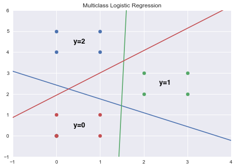
plt.title('Multiclass Logistic Regression')
plt.show()
Below is the plot of all the decision boundaries found by the logistic regression.
Value of \(h_\theta^{(i)}(x)\) is the probability of data point belonging to \(i^{th}\) class as seen in (1). Keeping this is mind one can decide the precedence of the class based on the values of its corresponding prediction on that data point. So, the predicted class is the one with maximum value of corresponding hypothesis. It shown in the plot below.
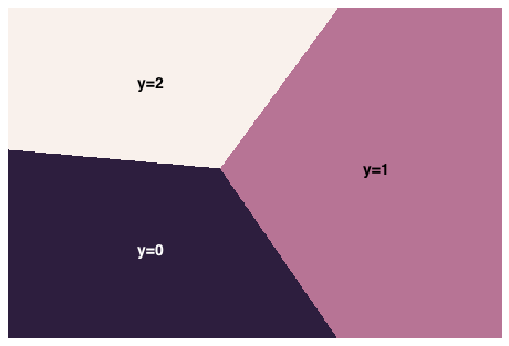
Similar to the above implementation the classificaiton can be extented to many more classes.
REFERENCES:
Machine Learning: Coursera - Multiclass Classification: One-vs-All