Basics of Machine Learning Series

Index

Overfitting

If the number of features is very high, then there is a probability that the hypothesis fill fit all the points in the training data. It might seem like a good thing to happen but has a contradictory results. Suppose a hypothesis of high degree is fit to a set of points such that all the points lie of the hypothesis. Plot below shows a case of overfitting with a regression of order 100.

This plot can be created if the code from Multivariate Linear Regression is run with the parameter order of regression set to 100.

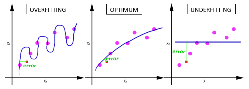
The curve above shows a case of overfitting where the hypothesis has high variance. While it fits the training data with good accuracy, it will fail to predict the values for unseen cases with same accuracy because of the high variance in the prediction curve.

Opposite to this spectrum is the case of underfitting. For example there exists a data set that increased linearly initialy and then saturates after a point. If a univariate linear regression is fit to the data it will give a straight line which might be the best fit for the given training data, but fails to recognize the saturation of the curve. Such a hypothesis is said to be underfit and have high bias i.e. the hypothesis is biased that the prediction should vary linearly over the feature variation. An optimum hypothesis is the trade off between variance and bias. All three cases can be seen in the plots below.

Both underfitting and overfitting are undesirable and should be avoided.

While overfitting might seem to work well for the training data, it will fail to generalize to new examples.

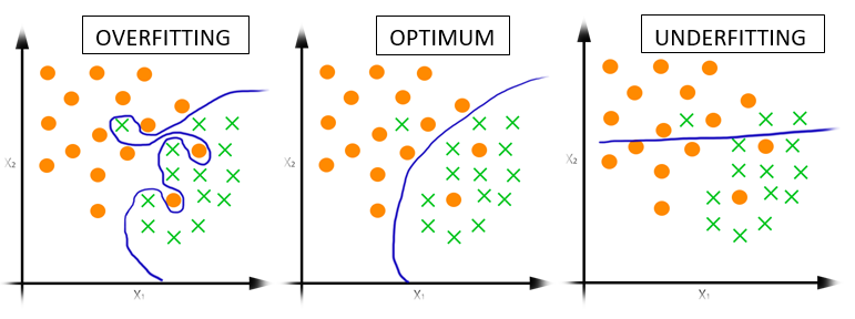
Overfitting and underfitting are not limited to linear regression but also affect other machine learning techniques. Effect of underfitting and overfitting on logistic regression can be seen in the plots below.

Detecting Overfitting

For lower dimensional datasets, it is possible to plot the hypothesis to check if is overfit or not. But same strategy cannot be applied when the dimensionality of the dataset increases beyond the limit of visualization. So, plotting hypothesis may not always work. So other methods have to utilized to address overfitting.

There are two options to avoid the overfitting:

• Reduce the number of features: Mostly overfitting is observed when the number of features is really high and the number of training examples are less. In such cases reducing the number of features can help avoid the issue of overfitting. Reducing the number of features can be done manually, or using model selection algorithms which help decide which features to eliminate. This also presents a disadvantage as removing features is sometimes equivalent to removing information.

• Regularization: Keep all the features but reduce magnitude/values of parameters \(\theta_j\). This technique works well, when there exists a lot features and each contributes a bit to the prediction, i.e. Regularization works well when there are a lot of slightly useful features.

Regularization Intuition

It is mathematically seen that the high variance of a overfit hypothesis is attributed to higher value of parameters corresponding to higher order features i.e. more the dependency is biased on a single feature, greater are the chances of a hypothesis overfitting. This effect can be counter acted by making sure that the values of parameter \(\theta_j\) are small. This is done by penalizing the algorithm proportional to value of \(\theta_j\) which will ensure small values of these parameters and hence would prevent overfitting by attributing small contributions from each features and hence removing high bias or high variance.

So the main ideas in regularization are:

• maintain small values for the parameters \(\theta_0, \theta_1, \cdots , \theta_n \)
  • which keeps the hypothesis simple
  • and less prone to overfitting

Mathematically, regularization is acheived by modifying the cost function as follows,

• Where \(\lambda \sum_{i=1}^n \theta_j^2\) is the regularization term and \(\lambda\) is called the regularization parameter. If noticed closely, this term mainly points to the fact that if value of \(\theta_j\) is increased, it would consequently increase the cost which is to be minimized during gradient descent. So it would ensure small values of the parameters as intented to prevent overfitting. By convention \(\theta_0\) is not penalized but in practice it does not affect the algorithm a lot.

• The regularization parameter \(\lambda\), controls the trade off between the goal of fitting the training set well and the goal of keeping the parameters small and the hypothesis simple. So, if the value of \(\lambda\) is kept very large, it would fail to fit the dataset properly and would give a underfit hypothesis.

REFERENCES:

Machine Learning: Coursera - The Problem of Overfitting
Machine Learning: Coursera - Cost Function