Basics of Machine Learning Series

Index

The intuition of regularization are explained in the previous post: Overfitting and Regularization. The cost function for a regularized linear equation is given by,

• Where
  • \(\lambda \sum_{i=1}^n \theta_j^2\) is the regularization term
  • \(\lambda\) is called the regularization parameter

Regularization for Gradient Descent

Previously, the gradient descent for linear regression without regularization was given by,

• Where \(j \in \{0, 1, \cdots, n\} \)

But since the equation for cost function has changed in (1) to include the regularization term, there will be a change in the derivative of cost function that was plugged in the gradient descent algorithm,

Because the first term of cost fuction remains the same, so does the first term of the derivative. So taking derivative of second term gives \(\frac {\lambda} {m} \theta_j\) as seen above.

So, (2) can be updated as,

• Where \(j \in \{1, 2, \cdots, n\} \)

It can be noticed that, for case j=0, there is no regularization term included which is consistent with the convention followed for regularization.

The second equation in the gradient descent algorithm above can be written as,

• Where \(\left(1 - \alpha {\lambda \over m} \right) \lt 1\) because \(\alpha\) and \(\lambda\) are both positive.

The implementation from Mulivariate Linear Regression can be updated with the following updated regularized functions for cost function, its derivative, and updates. One, can notice that \(theta_0\) has not been handled seperately in the code. And as expected it does not affect the regularization much. It can be implemented in the conventional way by adding a couple of logical expressions to the function

"""
Regularized Version
"""
def reg_j_prime_theta(data, theta, l, order_of_regression, i):
    result = 0
    m = len(data)
    for x, y in data :
        x = update_features(x, order_of_regression)
        result += (h(x, theta) - y) * x[i]
    result += l*theta[i]
    return (1/m) * result

def reg_j(data, theta, l, order_of_regression):
    cost = 0
    m = len(data)
    for x, y in data:
        x = update_features(x, order_of_regression)
        cost += math.pow(h(x, theta) - y, 2)
    reg = 0
    for j in theta:
        reg += math.pow(j, 2)
    reg = reg * l
    return (1/(2*m)) * (cost + reg)

def reg_update_theta(data, alpha, theta, l, order_of_regression):
    temp = []
    for i in range(order_of_regression+1):
        temp.append(theta[i] - alpha * reg_j_prime_theta(data, theta, l, order_of_regression, i))
    theta = np.array(temp)
    return theta

def reg_gradient_descent(data, alpha, l, tolerance, theta=[], order_of_regression = 2):
    if len(theta) == 0:
        theta = np.atleast_2d(np.random.random(order_of_regression+1) * 100).T
    prev_j = 10000
    curr_j = reg_j(data, theta, l, order_of_regression)
    print(curr_j)
    cost_history = []
    theta_history = [] 
    counter = 0
    while(abs(curr_j - prev_j) > tolerance):
        try:
            cost_history.append(curr_j)
            theta_history.append(theta)
            theta = reg_update_theta(data, alpha, theta, l, order_of_regression)
            prev_j = curr_j
            curr_j = reg_j(data, theta, l, order_of_regression)
            if counter % 100 == 0:
                print(curr_j)
            counter += 1
        except:
            break
    print("Stopped with Error at %.5f" % prev_j)
    return theta, cost_history, theta_history
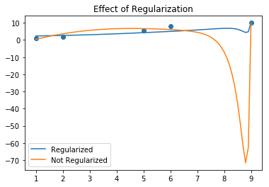
reg_theta, reg_cost_history, reg_theta_history = reg_gradient_descent(data, 0.01, 1, 0.0001, order_of_regression=150)

The following plot is obtained on running a random experiment with regression of order 150, which clearly shows how the regularized hypothesis is much better fit to the data.

Regularization for Normal Equation

The equation and derivation of Normal Equation can be found in the post Normal Equation. It is given by,

But after adding the regularization term as shown in (1), making very small changes in the derivation in the post, one can reach the result for regularized normal equation as shown below,

• Where
  • I is the identity matrix
  • \(L = \begin{bmatrix} 0 & 0 & \cdots & 0 \\ 0 & 1 & \cdots & 0 \\ \vdots & \vdots & \ddots & \vdots \\ 0 & 0 & \cdots & 1 \\ \end{bmatrix} \) is a square matrix of size (n+1)

If \(m \le n\), then the \(X^TX\) was non-invertible in the unregularized case but, \(X^TX + \lambda I\) does not face the same issues and is always invertible.

The effect of regularization on regression using normal equation can be seen in the following plot for regression of order 10.

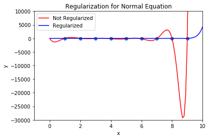
No implementation of regularized normal equation presented as it is very straight forward.

REFERENCES:

Machine Learning: Coursera - Regularized Linear Regression