Neural Networks: Cost Function and Backpropagation

Intuition behind the idea of backpropagation and its extension to calculate cost function

· · ·

Basics of Machine Learning Series

Index

· · ·

Notation

${(x^{(1)}, y^{(1)}), (x^{(2)}, y^{(2)}), \cdots , (x^{(m)}, y^{(m)})}$ are the $m$ training examples
L is the total number of the layers in the network
$s_l$ is the number of units (not counting the bias unit) in the layer l
K is the number of units in the output layer

Neural Network Notations

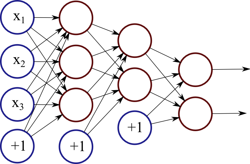
For example in the network shown above,
- L = 4
- $s_1 = 3,\, s_2 = 3,\, s_3 = 2,\, s_4 = 2$
- K = 2

One vs All method is only needed if number of classes is greater than 2, i.e. if $K \gt 2$, otherwise only one output unit is sufficient to build the model.

Cost Function of Neural Networks

Cost function of a neural network is a generalization of the cost function of the logistic regression. The L2-Regularized cost function of logistic regression from the post Regularized Logistic Regression is given by,

$J(\theta) = -{1 \over m} \sum_{i=1}^m \left( y^{(i)}\,log(h_\theta(x^{(i)})) + (1-y^{(i)})\,log(1 - h_\theta(x^{(i)})) \right) + {\lambda \over 2m } \sum_{j=1}^n \theta_j^2 \tag{1} \label{1}$

Where
- ${\lambda \over 2m } \sum_{j=1}^n \theta_j^2$ is the regularization term
- $\lambda$ is the regularization factor

Extending (1) to then neural networks which can have K units in the output layer the cost function is given by,

$J(\theta) = -{1 \over m} \left[ \sum_{i=1}^m \sum_{k=1}^K y_k^{(i)}\,log(h_\theta(x^{(i)}))_k + (1-y_k^{(i)})\,log(1 - (h_\theta(x^{(i)}))_k) \right] + {\lambda \over 2m } \sum_{l=1}^{L-1} \sum_{i=1}^{s_l} \sum_{j=1}^{s_{l+1}} (\theta_{ji}^{(l)})^2 \tag{2} \label{2}$

Where
- $h_\Theta(x) \in \mathbb{R}^K $
- $(h_\theta(x))_i$ is the $i^{th}$ output

Here the summation term $\sum_{k=1}^K$ is to generalize over the K output units of the neural network by calculating the cost function and summing over all the output units in the network. Also following the convention in regularization, the bias term in skipped from the regularization penalty in the cost function defination. Even if one includes the index 0, it would not effect the process in practice.

% y_vec is the target vector in one-hot encoded matrix form
% y_hat is the prediction from the network after forward propagation
J = ones(1, m) * ((- (y_vec .* log(y_hat)) - ((1 - y_vec) .* log(1 - y_hat))) * ones(k, 1)) / m;

% vectorized implementation of regularization terms
% note that (2:end) ensures that the biases are not regularized
% which is also seen the equations (2) above
reg_Theta1 = ones(1, size(Theta1, 1)) * ((Theta1 .* Theta1)(:, 2:end) * ones(size(Theta1, 2)-1, 1));
reg_Theta2 = ones(1, size(Theta2, 1)) * ((Theta2 .* Theta2)(:, 2:end) * ones(size(Theta2, 2)-1, 1));

% final cost with regularization
J = J + (lambda / (2*m) * (reg_Theta1 + reg_Theta2));

Backpropagation Algorithm

Backpropagation algorithm is based on the repeated application of the error calculation used for gradient descent similar to the regression techniques, and since it is repeatedly applied in the reverse order starting from output layer and continuing towards input layer it is termed as backpropagation.

For a network with L layers the computation during foward propagation, for an input $(x, y)$ would be as follows,

$\begin{align} a^{(1)} &= x \\ z^{(2)} &= \Theta^{(1)}\,a^{(1)} \\ a^{(2)} &= g(z^{(2)}) \qquad (add\, a_0^{(2)})\\ & \vdots \\ a^{(L-1)} &= g(z^{(L-1)}) \qquad (add\, a_0^{(L-1)})\\ z^{(L)} &= \Theta^{(L-1)}\,a^{(L-1)} \\ a^{(L)} &= h_\Theta(x) = g(z^{(L)}) \end{align}$

The $h_\Theta(x)$ is the prediction. In order to reduce the error between the prediction and the actual value backpropagation is used. Say, $\delta_j^{(l)}$ is the error of node j in the layer l is associated with the prediction made at that node given by $a_j^{(l)}$, then backpropagation aims to calculate this error term propating backwards starting from the output unit in the last layer (layer L in the example above).

So for each output unit in layer L, the error term is given by, $\delta_j^{(L)} = a_j^{(L)} - y_j$ which can be vectorized and written as,

$\delta^{(L)} = a^{(L)} - y \tag{3} \label{3}$

Where $a^{(L)}$ is $h_\Theta(x)$.

Now the error terms for the previous layers are calculated as follows,

$\delta^{(l)} = (\Theta^{(l)})^T\,\delta^{(l+1)} .* g'(z^{(l)}) \tag{4} \label{4}$

Where
- $g’(z^{(l)}) = a^{(l)} .* (1 - a^{(l)}) $
- .* is the element-wise multiplication.

This backward propagation stops at l = 2 because l = 1 correponds to the input layer and no weights needs to be calculated there.

Now the the gradient for the cost function which is needed for the minimization of the cost function is given by,

$\frac {\partial J} {\partial \Theta_{ij}^{(l)} } = a_j^{(l)}\, \delta_i^{(l+1)} \tag{5} \label{5}$

Where regularization is ignored for the simplicity of expression.

Summarizing backpropagation:

Given training set ${(x^{(1)}, y^{(1)}), \cdots, (x^{(m)}, y^{(m)})}$

Set $\Delta_{ij}^{l} = 0$ for all (i, j, l)
For i = 1 to m:
- Set $a^{(1)} = x^{(i)} $
- Perform forward propagation to compute $a^{(l)}$ for l = 1, …, L
- Using $y^{(i)}$ compute $ \delta^{(L)} = a^{(L)} - y^{(i)} $
- Compute $\delta^{(L-1)}, \cdots, \delta^{(2)}$ using backpropagation
- $\Delta_{ij}^{(l)} := \Delta_{ij}^{(l)} + a_j^{(l)} \delta_i^{(l+1)} $

Vectorized implementation of the equation above is given by,

$\Delta^{(l)} := \Delta^{(l)} + \delta^{(l+1)}\,(a^{(l)})^T \tag{6} \label{6}$

$D_{ij}^{(l)} := {1 \over m} \Delta_{ij}^{(l)} + \lambda \, \Theta_{ij}^{(l)} $ if $j \ne 0$
$D_{ij}^{(l)} := {1 \over m} \Delta_{ij}^{(l)} $ if $j = 0$
And finally, $ \frac {\partial} {\partial \Theta_{ij}^{(l)} } = D_{ij}^{(l)} $

% example of backward propgation of error signal
del_3 = y_hat - y_vec;
del_2 = (del_3 * Theta2)(:, 2:end) .* sigmoidGradient(z2);

% calculation of partial derivatives from the error signals
Theta2_grad = (del_3' * a2) / m;
Theta1_grad = (del_2' * a1) / m;

% calculation of regularization parameters
% (2:end) ensures no regularization of biases
% as seen in equation (6)
Theta2_grad(:, 2:end) = Theta2_grad(:, 2:end) + lambda * Theta2(:, 2:end) / m;
Theta1_grad(:, 2:end) = Theta1_grad(:, 2:end) + lambda * Theta1(:, 2:end) / m;

The capital delta matrix $D$, is used as an accumulator to add up the values as backpropagation proceeds and finally compute the partial derivatives.

The complete vectorized implementation for the MNIST dataset using vanilla neural network with a single hidden layer can be found here.

Backpropagation Intuition

Say $(x^{(i)}, y^{(i)})$ is a training sample from a set of training examples that the neural network is trying to learn from. If the cost function is applied to this single training sample while setting $\lambda = 0$ for simplicity, then \eqref{2} can be reduced to,

$J(\Theta) = - {1 \over m} \left [ \sum_{i=1}^m y^{(i)} log(h_\Theta(x^{(i)})) + (1-y^{(i)}) log(1-h(_\Theta(x^{(i)}))) \right ]$

where,

$cost(i) = y^{(i)} log(h_\Theta(x^{(i)})) + (1-y^{(i)}) log(1-h(_\Theta(x^{(i)}))) \tag{7} \label{7}$

which is very similar to the cost for a logistic regression, which can also be seen analogous to the cost for a linear regression (mean-squared error), i.e.

$cost(i) \approx (h_\Theta(x^{(i)}) - y^{(i)})^2$

This basically gives a magnitude of how well the network is doing in prediction of the output for a single training sample.

Formally, the $\delta$ terms are the partial derivatives of the cost function given by,

$\delta_j^{(l)} = \frac {\partial} {\partial z_j^{(l)}} cost(i) \tag{8} \label{8}$

where $cost(i)$ is given by \eqref{7}.

So, \eqref{8} conveys mathematically the intent to change the cost function (by changing the network parameters), in order to effect the intermediate values calculated in $z’s$, so as to minimize the differences in the final output of the network.

The basis of backpropagation is benched on the propagating the error term calculated for the final layer using \eqref{3} and \eqref{4} backwards to the preceding layers.

For more on mathematics of backpropagation, refer Mathematics of Backpropagation. For an approximate implementation of backpropagation using NumPy and checking results using Gradient Checking technique refer Backpropagation Implementation and Gradient Checking.

REFERENCES:

Machine Learning: Coursera - Cost Function

· · ·

Shams S

AIML Resident @ Apple

Neural Networks: Cost Function and Backpropagation

Intuition behind the idea of backpropagation and its extension to calculate cost function

Basics of Machine Learning Series

Notation

Cost Function of Neural Networks

Backpropagation Algorithm

Backpropagation Intuition

REFERENCES:

Notes

Recursing the Rabbit Hole