Prerequisites

• Python Programming
• Basics of Arrays
• Basics of Machine Learning

TensforFlow APIs

• The lowest level TensorFlow API, TensorFlow Core, provides the complete programming control, recommended for machine learning researchers who require fine levels of control over their model.
• The higher level TensorFlow APIs are built on top of TensorFlow Core. These APIs are easier to learn and use. Higher level APIs also provide convinient wrappers for repetitive tasks, e.g. tf.estimator helps to manage datasets, estimators, training, inference etc.

Terminologies

• Computational Graph defines the series of TensorFlow operations arranged in the form of graph nodes.
• Dataset: Similar to placeholders, but Dataset represents a potentially large set of elements that can be accessed using iterators. These are the preferred method of streaming data into a model.
• Node in a TensorFlow graph takes zero or more tensors as inputs and produces a tensor as an output, e.g. Constant is a type of node in TensorFlow that takes no inputs and outputs the value that it stores internally (as defined in the defination of Tensorflow nodes earlier).
• Operations are another kind of node in TensorFlow used to build the computational graphs, that consume and produce tensors.
• Placeholder is a promise to provide value later. These serve the purpose or parameters or arguments to a graph which represents a dynamic function based on inputs.
• Rank: The number of dimensions of a tensor (similar to rank of a matrix).
• Session, used for evaluation of TensorFlow graphs, encapsulates the control and state of the TensorFlow runtime.
• Shape: Often confused with rank, shape refers to the tuple of integers specifying the length of tensor along each dimension.
• Tensor: A set of primitive types shaped into an array of any number of dimensions. It can be considered a higher-dimensional vector. Tensorflow used numpy arrays to represent tensor values.
• TensorBoard is a TensorFlow utility used to visualize the computational graphs.

TensorFlow Imports

from __future__ import absolute_import
from __future__ import division
from __future__ import print_function

import numpy as np
import tensorflow as tf

• absolute_import: The distinction between absolute and relative imports can be considered to be analogous to the concept of absolute or relative file paths or even URLs, i.e. absolute imports specify the exact path of the imports while the relative imports work w.r.t. the working directory. Therefore for the code that is to be shared among peers, it is recommended to use absolute imports.

• division: The import belongs to era when the debate on true division vs floor division was on in the python community i.e. for python 2.*. The import in python 3.* is not required as the regular division operator itself is the true division while the floor division is denoted by \\.

• print_function: This import is again not necessary in python 3.*. It is used to invalidate the print as a statement in python 2.*. Post call to this function, print only has valid represetnation as a function, which has some apparent advantages over the print as a statement, e.g. print function can be used inside lambda function or list and dictionary comprehensions.

Generally all the __future__ imports are recommended to be kept at the top of the file because it changes the way the compiler behaves and the set of rules it follows.

Initialization

Basically, a TensorFlow Core program can be split into two sections:

• Building the computational graph
• Running the computational graph

Tensor initialization is done as follows:

import tensorflow as tf
a = tf.constant(3.0, 
                dtype=tf.float32, 
                name='a')
b = tf.constant(4.0, 
                name='b')
print(a)
print(b)

The output shows that the default type of a tensor is float32.

Tensor("a:0", shape=(), dtype=float32)
Tensor("b:0", shape=(), dtype=float32)

Also, the print statement does not print value assigned to the nodes. The actual values will be displayed only on evaluation of the nodes. In TensorFlow the evaluation of a node can only be done within a session as shown below.

Session

sess = tf.Session()
sess.run([a, b])

More complex TensorFlow graphs are built using operation nodes. For example,

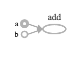
total = tf.add(a, b)
print(total)
sess.run(total)

Mutliple tensors can be passed to a tf.Session.run, i.e., the run method handles any combination of tuples dictionaries,

sess.run({'ab': (a, b), 'total': total})

Some tensorflow functions return tf.Operations instead of tf.Tensors. Also, the result of calling run on an Operation is None because Operations are run to cause a side-effect and not to retrieve a value.

During a call to tf.Session.run, and tf.Tensor holds a single value throughout that run. This is consistent with the notion that state of graph is saved in a session making sure once initialized a tensor will not have updated values unless operated upon.

TensorBoard

In order to visualize the TensorFlow graph, following command can be followed:

tf.summary.FileWriter('/path/to/save/', sess.graph)

or

writer = tf.summary.FileWriter('/path/to/save')
writer.add_graph(tf.get_default_graph())

Now run the following command on the terminal, ensure TensorBoard is installed.

tensorboard --logdir=/path/to/save

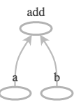
It leads to the above graph displayed, which is an apt representation of the minimal graph that has been built so far. But it is a constant graph as the input nodes are constants. In order to build a parameterized graph, placeholders are used as shown below.

Feeding Data using Placeholders

a = tf.placeholder(tf.float32, name='a')
b = tf.placeholder(tf.float32, name='b')
z = a+b

sess = tf.Session()
print(sess.run(z, {a: 3, b: 4}))
print(sess.run(z, feed_dict={a: [1, 2, 3], b: [4, 5, 6]}))

tf.summary.FileWriter('/path/to/save', sess.graph)

The feed_dict argument can be used to overwrite any tensor in the graph.

The only difference between placeholders and other tf.Tensors is that placeholders throw and error if no value is fed to them.

run(
    fetches,
    feed_dict=None,
    options=None,
    run_metadata=None
)

Runs operations and evaluates tensors listed in fetches argument. The method will run one step of TensorFlow computation, by running necessary graph consisting of tensors and operations to evaluate the dependencies of Tensors listed in fetches, substituting the values listed in the feed_dict for the corresponding values.

The fetches argument can be a single graph element, nested list, tuple, namedtuple, dict, or OrderedDict that consists of graph elements as its leaves.

The graph element may belong to one of the following classes:

• tf.Operation: fetched value is None.
• tf.Tensor: fetched value is a numpy ndarray containing the value of the tensor.
• tf.SparseTensor: fetched value is a tf.SparseTensorValue.
• get_tensor_handle op: fetched value is a numpy ndarray containing the handle of the tensor.
• string: name of a tensor or operation in the graph.

The value returned by run() has the same shape as the fetches argument, where leaves are replaced by corresponding values returned by TensorFlow.

Example code:

import collections
a = tf.constant([10, 20])
b = tf.constant([1.0, 2.0])
data = collections.namedtuple('data', ['a', 'b'])
v = sess.run({'k1': data(a, b), 'k2': [b, a]})
print(v)

It can be observed on executing the code that the output of run saved has the same structure as the input to the fetches argument, i.e. a dictionary of namedtuple of lists and list of lists.

The keys in feed_dict can belong to one of the following:

• If key is tf.Tensor: value maybe a scalar, string, list, or numpy array.
• If key is tf.Placeholder: shape of the value will be checked with shape of the placeholder for compatibility.
• If key is tf.SparseTensor: value should be tf.SparseTensorValue.
• If key is nested tuple of Tensors or SparseTensors, then the value should be follow the same nested structure that maps to corresponding values in the key’s structure.

Each value in the feed_dict must be convertible to a numpy array of the dtype of corresponding key.

The following errors are raised by run function:

• RuntimeError: If the Session is in invalid state or closed.
• TypeError: If fetches or feed_dict keys are of inappropriate types.
• ValueError: If fetches or feed_dict keys are invalid or refer to a tensor that does not exist.

Importing Data

tf.data api helps to build complex input pipelines. It basically helps deal with large amounts of data, maybe belonging to different formats and apply complicated transformations to the data such as image augmentation or handling text sequences of different lengths for preprocessing and batch processing use cases. The pipelines help abstract processes and also modularize the code for easier debugging and managing of the code.

Some of the abstractions dataset introduces in TensorFlow are summarized below:

• tf.data.Dataset is used to represent a sequence of elements where each element contains one or more Tensor objects.

Creating a source (Dataset.from_tensor_slices()) contructs a dataset from one or more tf.Tensor objects, while applying a transformation (Dataset.batch()) contructs a dataset from one or more tf.data.Dataset objects.

• tf.data.Iterator is used to extract elements from a dataset, and acts as an interface between the input pipeline and the models.

The get_next method of iterator is called for streaming the data.

Simplest iterator is made using make_one_shot_iterator method as shown below. It is associated with a particular dataset and iterates through it once.

data = [
    [0, 1,],
    [2, 3,],
    [4, 5,],
    [6, 7,],
]
slices = tf.data.Dataset.from_tensor_slices(data)
next_item = slices.make_one_shot_iterator().get_next()
while True:
  try:
    print(sess.run(next_item))
  except tf.errors.OutOfRangeError:
    break

Reaching the end of dataset, if get_next is called, OutOfRangeError is thrown by the Dataset.

For more sophisticated uses, Iterator.initializer is used that helps reinitialize and parameterize an iterator with different datasets, including running over a single or a set of datasets multiple number of times in the same program.

Placeholders work for simple experiments, but Datasets are the preferred method of streaming data into a model.

A dataset consists of elements that each have exactly the same structure, i.e. an element contains one or more tf.Tensor objects, called components. A component has tf.DType representing the type of elements in the tensor, and a tf.TensorShape (maybe partially specified, for example batch size might be missing but dimension of elements in batch may be present) representing the static shape of each element.

Similarly the Dataset.output_types and Dataset.output_shapes inspect the inferred types and shapes of each component of the dataset element.

It is optional but often helps to name the components in a dataset element. To summarize, one can use tuples, collections.namedtuples or a dictionary mapping strings to tensors to represent a single element in a Dataset.

Sample code to see the above properties:

def print_dtype(input_data, print_string=""):
    if type(input_data) == tuple:
        print_string += "("
        for _ in input_data:
            print_string = print_tuple(_, print_string)
        print_string += ")"
    else:
        print_string += str(input_data.dtype) + ", "
    return print_string

def print_dimension(input_data, print_string=""):
    if type(input_data) == tuple:
        print_string += "("
        for _ in input_data:
            print_string = print_dimension(_, print_string)
        print_string += ")"
    else:
        print_string += str(input_data.get_shape()) + ", "
    return print_string

dataset1 = tf.data.Dataset.from_tensor_slices(tf.random_uniform([4, 10]))
element1 = dataset1.make_initializable_iterator().get_next()
print("dataset1:")
print("\t", print_dtype(element1))
print("\t", print_dimension(element1))
print("\t", dataset1.output_types)
print("\t", dataset1.output_shapes)

dataset2 = tf.data.Dataset.from_tensor_slices(
   (tf.random_uniform([4]),
    tf.random_uniform([4, 100], maxval=100, dtype=tf.int32)))
element2 = dataset2.make_initializable_iterator().get_next()
print("dataset2:")
print("\t", print_dtype(element2))
print("\t", print_dimension(element2))
print("\t", dataset2.output_types)
print("\t", dataset2.output_shapes)

dataset3 = tf.data.Dataset.zip((dataset1, dataset2))
element3 = dataset3.make_initializable_iterator().get_next()
print("dataset3:")
print("\t", print_dtype(element3))
print("\t", print_dimension(element3))
print("\t", dataset3.output_types)
print("\t", dataset3.output_shapes)

Outputs:

dataset1:
    <dtype: 'float32'>, 
    (10,), 
    <dtype: 'float32'>
    (10,)
dataset2:
    (second:<dtype: 'int32'>, first:<dtype: 'float32'>, )
    (second:(100,), first:(), )
    {'second': tf.int32, 'first': tf.float32}
    {'second': TensorShape([Dimension(100)]), 'first': TensorShape([])}
dataset3:
    (d1:<dtype: 'float32'>, (second:<dtype: 'int32'>, first:<dtype: 'float32'>, ))
    (d1:(10,), (second:(100,), first:(), ))
    {'d1': tf.float32, 'd2': {'second': tf.int32, 'first': tf.float32}}
    {'d1': TensorShape([Dimension(10)]), 'd2': {'second': TensorShape([Dimension(100)]), 'first': TensorShape([])}}

So, the basic mechanics of import data can be listed as follows:

• Define a source is the first step in defining an input pipeline. For example, data can be imported from in-memory tensors using tf.data.Dataset.from_tensors() or tf.data.Dataset.from_tensor_slices(). It can also be imported from disk if the data is in recommended TFRecord format using tf.data.TFRecordDataset

• Transformations can be applied on any dataset to obtain subsequent dataset objects. This can be achieved by chaining preprocessing or transformation operations. For example, per-element transformations can be applied using Dataset.map() or multi-element transformations can be applied using Dataset.batch().

Dataset transformations support datasets of any structure. The element structure determines the argument of a function. For example,

dataset1 = dataset1.map(lambda x: ...)

dataset2 = dataset2.flat_map(lambda x, y: ...)

dataset3 = dataset3.filter(lambda x, (y, z): ...)

From the example above it can be seen that the lambda function can take any structure as the input based on the structure of an element in the dataset, however complex it is.

• Define an iterator to stream data into the model. The iterator can be one-shot iterator as in the example above or one of the types listed below.

  • One-shot iterator is the simplest iterator that supports iterating only once through the dataset and does not require an explicit initialization. Hence, as a by-product, it does not allow parameterization.

  • Initializable iterator requires an explicit iterator.initializer operation before using it. At the cost of this inconvinience, it gives the flexibility to parameterize the defination of dataset using placeholders.

max_value = tf.placeholder(tf.int64, shape=[])
dataset = tf.data.Dataset.range(max_value)
iterator = dataset.make_initializable_iterator()
next_element = iterator.get_next()

# parameter passing for the placeholder
sess.run(iterator.initializer, feed_dict={max_value: 10})
for i in range(10):
  value = sess.run(next_element)
  assert i == value

• Reinitializable iterator can be initialized from multiple different dataset objects. Basically, while the datasets may change they have the same structure attributed to each element of the dataset. A reinitializable iterator is defined by its structure and any dataset complying to that structure can used to initialize the iterator.

# two different datasets with same structure
training_dataset = tf.data.Dataset.range(100).map(
    lambda x: x + tf.random_uniform([], -10, 10, tf.int64))
validation_dataset = tf.data.Dataset.range(50)

# define the iterator using the structure property
iterator = tf.data.Iterator.from_structure(training_dataset.output_types,
                                           training_dataset.output_shapes)
next_element = iterator.get_next()

training_init = iterator.make_initializer(training_dataset)
validation_init = iterator.make_initializer(validation_dataset)

# initialize for training set
sess.run(training_init)
sess.run(next_element)

# reinitialize for validation set
sess.run(validation_init)
sess.run(next_element)

• Feedable iterator is used along with tf.placeholder to select Iterator to use in each call of tf.Session.run, via the feed_dict mechanism. It does not require one to initialize the iterator from the start of a dataset when switching between the iterators. The tf.data.Iterator.from_string_handle can be used to define a feedable iterator.

string_handle = tf.placeholder(tf.string, shape=[])
iterator = tf.data.Iterator.from_string_handle(
    string_handle, 
    training_dataset.output_types, 
    training_dataset.output_shapes
)
next_element = iterator.get_next()

# get string handles of each iterator
training_handle = sess.run(training_iterator.string_handle())
validation_handle = sess.run(validation_iterator.string_handle())

# using training iterator
sess.run(next_element, feed_dict={string_handle: training_handle})

# using validation iterator
sess.run(next_element, feed_dict={string_handle: validation_handle})

Layers

A trainable model is implemented in TensorFlow by means of using Layers which adds trainable parameters to a graph. A layer packages the variables and the operations that act on them. For example, densely-connected layer performs weighted sum across all inputs from each output and applies an optional activation function. The connection weights and biases are managed by the layer object.

In order to apply layer to an input, the layer is called as a function with input as an argument.

After calling the layer as a function, based on the inputs to the layer it sets up shape of weight matrices compatible with the input. Now, the layers contain variables that must be initialized before they can be used.

import tensorflow as tf
x = tf.placeholder(tf.float32, shape=[None, 3], name='x')
linear_model = tf.layers.Dense(units=1, name='dense_layer')
y = linear_model(x)
init = tf.global_variables_initializer()
sess = tf.Session()
sess.run(init)
sess.run(y, {x: [[1, 2, 3],[4, 5, 6]]})

Calling tf.global_variables_initializer only creates and returns a handle to tensorflow operation which will initialize all global variables on call of tf.Session.run.

For each layer class (like tf.layers.Dense) there exists a shortcut function in TensorFlow (like tf.layers.dense) that creates and runs the layer in a single call. But this approach allows no access for the tf.layers.Layer object which might cause difficulties in debugging and introspection or layer reuse possibilities.

The graph of a linear model looks as shown below.

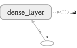
where the linear_model block internally has the structure as shown in Fig. 4 which abides by \eqref{1}.

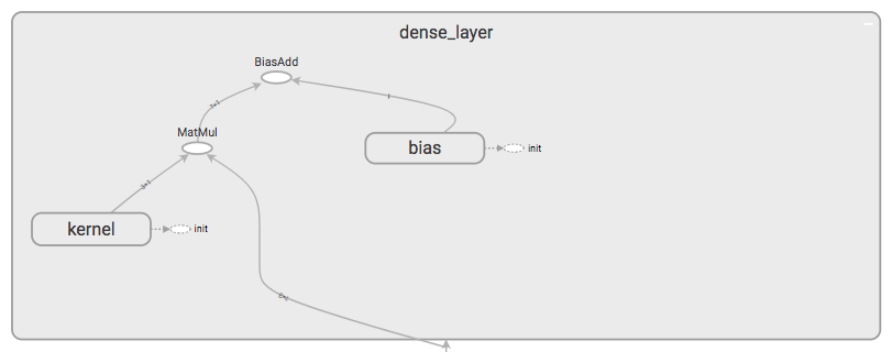
where W is the weights being fed by the kernel, x is the input vector being fed by the input placeholder and b is the bias.

Feature columns can be experimented with using tf.feature_column.input_layer function for dense columns as input and tf.feature_column.indicator_column for categorical indicators as input.

features = {
    'sales' : [[5], [10], [8], [9]],
    'department': ['sports', 'sports', 'gardening', 'gardening']}

department_column = tf.feature_column.categorical_column_with_vocabulary_list(
        'department', ['sports', 'gardening'])
department_column = tf.feature_column.indicator_column(department_column)

columns = [
    tf.feature_column.numeric_column('sales'),
    department_column
]

inputs = tf.feature_column.input_layer(features, columns)

var_init = tf.global_variables_initializer()
table_init = tf.tables_initializer()
sess = tf.Session()
sess.run((var_init, table_init))
print(sess.run(inputs))

Feature columns can have internal state, like layers and so need to be initialized. Similarly, categorical columns use lookup tables internally and hence require tf.table_initializer additionally.

Categorical input fed using indicator vectors are one-hot encoded.

Training

• Define the data and labels.

x = tf.constant([[1], [2], [3], [4]], dtype=tf.float32)
y_true = tf.constant([[2], [4], [6], [8]], dtype=tf.float32)

• Define the model

y_pred = tf.layers.dense(x, units=1)

At this point, model output can be evaluated

# initialize session and variable
sess = tf.Session()
init = tf.global_variables_initializer()
sess.run(init)

# extract model output
sess.run(y_pred)

The output would not be correct as the model is not trained to optimize model parameters for accuracy.

• To optimize the model, a loss has to be defined.

Using mean squared error,

loss = tf.losses.mean_squared_error(
    labels=y_true, 
    predictions=y_pred)

sess.run(loss)

• After defining a loss, one of the optimizers provided by TensorFlow out of box can be used as optimization algorithm.

The optimizers are defined in tf.train.Optimizer. Using the simplest gradient descent implemented in tf.train.GradientDescentOptimizer,

Gradient Descent modifies each variable according to the magnitude of the derivative of loss with respect to that variable.

optimizer = tf.train.GradientDescentOptimizer(0.01)
train = optimizer.minimize(loss)

• Training the model

At this stage the model graph is built and the only task pending is to call the evaluate train iteratively to minimize loss by optimizing model trainable parameters by updating the corresponding variables.

for i in range(100):
  _, loss_value = sess.run((train, loss))

• Evaluate model predictions

predictions = session.run(y_pred)

• Model Graph

The model graph generated from the above training example can be seen below.

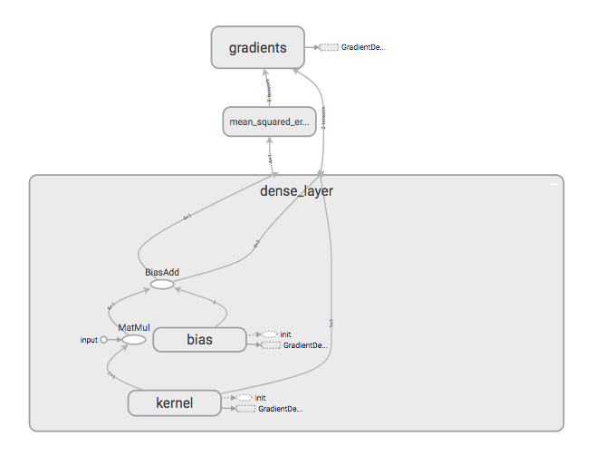
Since the model inputs are constants, it can be seen that the dense layer in the graph has no input being fed from outside, rather is a part of the dense block.

REFERENCES:

TensorFlow Low-level Introduction