Basics to Computer Vision Series

Index

Images as Function

Images are generally associated with concepts of vision and perception. But in the field of computer vision it is important to understand that image can be represented as a function as well. An image can be represented as a function \(I(x, y)\) which gives the intensity represented by height of the bar for a given coordinate \(x\) and \(y\).

So basically, an image can be thought of as one of the following:

• a matrix of numbers
• pixel intensity as a function of coordinates
• output of a camera

Theoretically, an image can be modelled as a function \(f\) or \(I\) from \(\mathbb{R}^2 \to \mathbb{R}\) where \(f(x,y)\) gives the intensity or value at position \((x,y)\).

Practically, an image can be modelled over a rectangle with a finite range, given by:

Similarly, color images are three functions stacked together representing the three channels (i.e. often R, G and B), written as, vector-valued functions (i.e. every pixel is a vector of numbers),

Such as function can be generalized as,

Digital Images

Another important realization in the computer vision is the fact that images in a computer system are discrete images and not continuous ones like human eyes see, i.e. images in computer have a matrix representation with non-continuous intensity values between two adjacent pixel which might not be the case for the actual ground truth image it is capturing.

Discretization of the digital image is two fold:

• Sample the actual image onto a 2D space of a regular matrix
• Quantize the intensity values (as digital images do not take continuous values for intensities) to the nearest integer.

Such operations often will lead to loss of some information but if often minimal and can be worked with.

Loading and Exploring Image

% import image and display
img = imread('tree.jpg');
imshow(img);

% load the image package
pkg load image;

% size of 3 channel image
disp(size(img));

% red channel extraction
img_red = img(:, :, 1);
imshow(img_red);
plot(img_red(80, :));

% convert to grayscale
gry = rgb2gray(img);

% size and class of image
disp(size(img));
disp(class(img));

% extract intensities from image
disp(gry(50, 100));
plot(gry(50, :));

• Slicing a matrix is same as cropping.

% cropping image by slicing
disp(gry(101:103, 201:203));

• Multiplying a matrix with a scalar (i.e scaling an image) helps adjust the brightness, i.e. if scalar greater than 1, the image becomes brighter else it gets darker because pixel value 255 represents white and 0 represents black.

% change brightness
function result = scale(image, value)
  result = image .* value;
endfunction

imshow(scale(img, 2));
imshow(scale(img, 0.5));

• Since images can be treated as functions and are represented as matrices, they can undergo matrix operations such as addition substraction.

% import test images
img_1 = imread('cycle.jpeg');
img_2 = imread('tree.jpg');

min_h = min(size(img_1)(1), size(img_2)(1));
min_w = min(size(img_1)(2), size(img_2)(2));

img_1 = img_1(1:min_h, 1:min_w, :);
img_2 = img_2(1:min_h, 1:min_w, :);

% add images
imshow(img_1 + img_2);
imshow(img_1./2 + img_2./2);

% difference of images
imshow(img_1 - img_2);
imshow(img_2 - img_1);
imshow(img_1 - img_2 + img_2 - img_1);

imshow(imabsdiff(img_1, img_2));

The default data type of image pixels in many environments (including octave and matlab) is 8-bit unsigned integer which has range [0, 255]. So special care must be taken during addition and subtraction because values can often go out of this range and be clipped at lower and higher limit.

• Alpha blending has roots in weighted addition of two images to maintain pixel limits within the range.

function result = blend(image_1, image_2, alpha)
  result = alpha .* image_1 + (1-alpha) .* image_2;
endfunction

imshow(blend(img_1, img_2, 0.75));
imshow(blend(img_1, img_2, 0.25));

The value \(\alpha\) and \((1 - \alpha)\) ensure that the pixel values during alpha blending does not overflow the limits of pixel intensities.

Noise in Image

Noise in an image can be represented with a function, i.e.

where \(\eta\) is the noise.

Common types of noise functions are:

• Salt and pepper noise is random occurences of white and black pixels.

imshow(imnoise(gry, 'salt & pepper', 0.1));

• Impulse noise has random occurences of white pixels only.
• Guassian noise has variations in intensity drawn from a Guassian normal distribution.

imshow(imnoise(gry, 'gaussian'));

noise = randn(size(gry)) .* 200;
imshow(gry + noise);

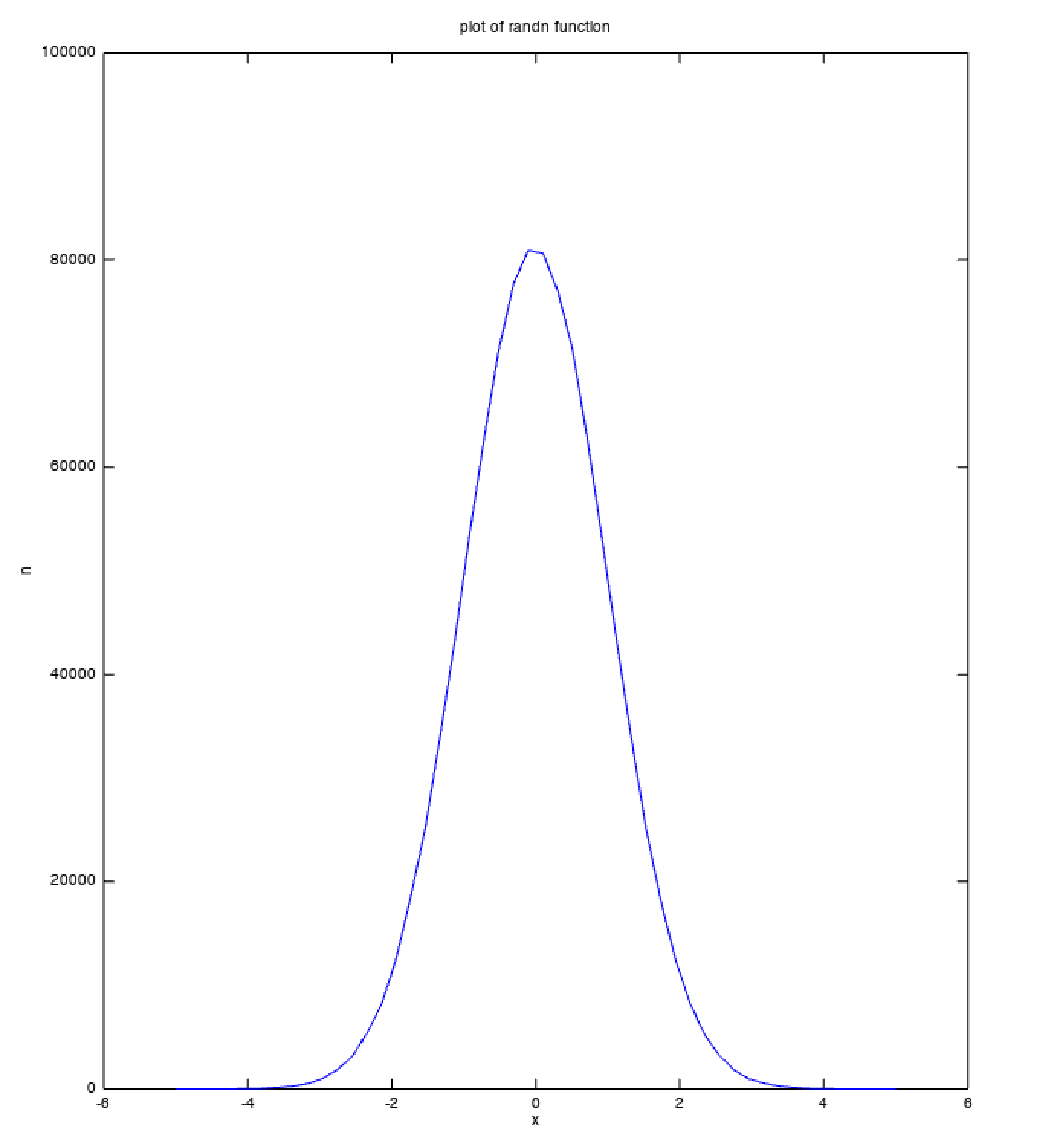
It is possible to check that the values produced by randn function follow a normal distribution by plotting the values produced by the function.

% plotting randn
noise = randn([1, 1000000]);
[n, x] = hist(noise, linspace(-5, 5, 50));
plot(x, n);
title('plot of randn function');
xlabel('x');
ylabel('n');

Filtering

Noise filtering is the process of eliminating or reducing the effect of noise from an image.

• Moving Average Filter or mean filter is one of the basic filtering techniques that tries to smooth a noisy image by means of averaging values over a window in the image. as the window size increases the smoothness of the curve will increase. This generally does not mean that the quality of the image will be improved as it can cause a blurring effect.

This averaging is based on the following assumptions:

1. The value of a pixel at position must be similar to the ones nearby, surrounding it.
2. The noise added to each pixel is independent of other noise values and hence would average to zero.

Since noise is basically an addition of a noise function to the image function, it can be argued that it is possible to remove noise by performing the additive inverse, i.e. subtract noise function and hence retrieve the original image. But the fallacy in such an argument lies in the fact that the noise functions are generally not reproducible and would not have a standard form associated with them. They might have a standard statistical form such as following a given probabilistic distribution.

Additive noise may also lead to loss of information if the value of pixels is scaled beyond the limits of the image pixel range.

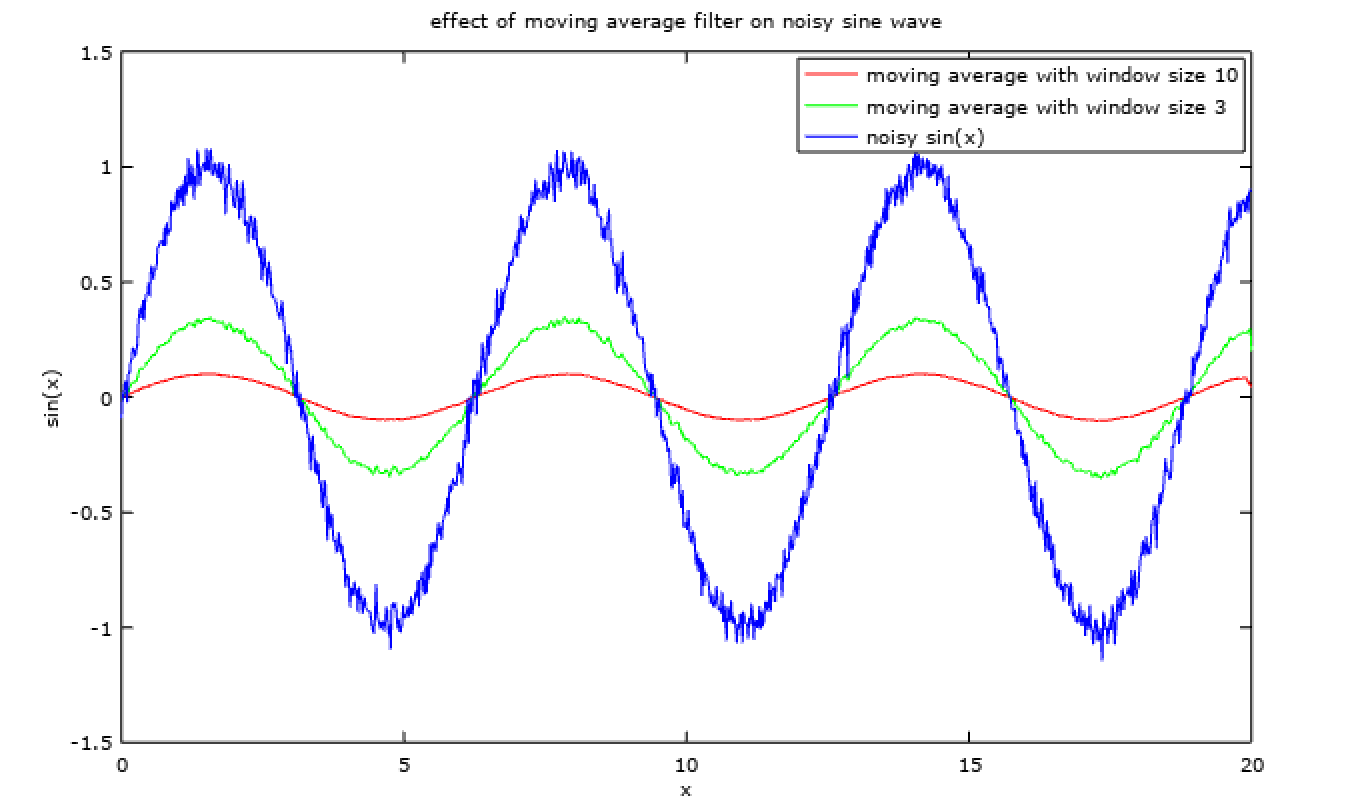
Effect of moving average filter can be seen on a noisy sine wave using basic octave operations,

% moving average filters 
f_3 = fspecial('average', 3);
f_10 = fspecial('average', 10);

% adding noise to sine wave
x = linspace(0, 20, 1000);
sin_x = sin(x);
noise = randn(size(sin_x)) .* 0.05;
sin_x_noisy = sin_x + noise;

% moving average filter on sin wave
sin_x_filtered_10 = imfilter(sin_x_noisy, f_10);
sin_x_filtered_3 = imfilter(sin_x_noisy, f_3);
plot(
  x, sin_x_filtered_10, 'r',
  x, sin_x_filtered_3, 'g',
  x, sin_x_noisy, 'b'
);
title('effect of moving average filter on noisy sine wave');
xlabel('x');
ylabel('sin(x)');
legend (
  'moving average with window size 10', 
  'moving average with window size 3',
  'noisy sin(x)'
);

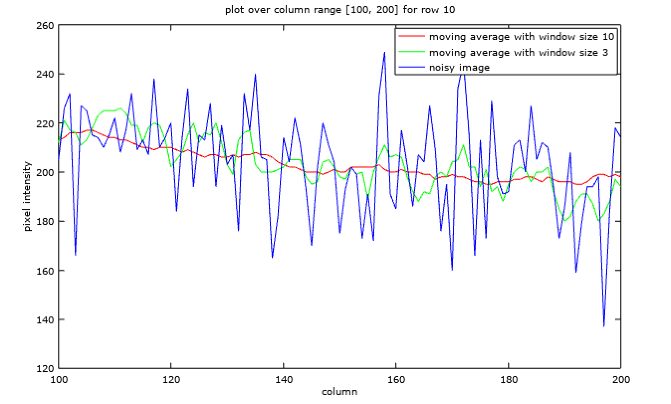
Similarly it can be applied to an image,

% import library
pkg load image;
img = imread('tree.jpg');
img = rgb2gray(img);
imshow(img);

% adding noise to image
sigma = 20;
noise = randn(size(img)) .* sigma;
img_noisy = img + noise;
imshow(img_noisy);

% moving average filter on image
img_filtered_3 = imfilter(img_noisy, f_3);
img_filtered_10 = imfilter(img_noisy, f_10);

x = linspace(100, 200, 101);
plot(
  x, img_filtered_10(10, 100:200), 'r', 
  x, img_filtered_3(10, 100:200), 'g', 
  x, img_noisy(10, 100:200), 'b'
);
title('plot over column range [100, 200] for row 10');
xlabel('column');
ylabel('pixel intensity');
legend (
  'moving average with window size 10', 
  'moving average with window size 3',
  'noisy image'
);


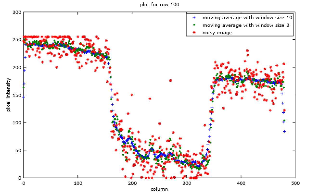
w = size(img)(2);
x = linspace(0, w, w);
plot(
  x, img_filtered_10(100, :), '+', 
  x, img_filtered_3(100, :), '.', 
  x, img_noisy(100, :), '*'
);
title('plot for row 100');
xlabel('column');
ylabel('pixel intensity');
legend (
  'moving average with window size 10', 
  'moving average with window size 3',
  'noisy image'
);

• Weighted Moving Average takes the assumption a step further than the moving average, positing that if a pixel is similar to nearby pixels then it should be more dependent on the nearer ones than on the farther ones. This information is encoded as weighted average for such filtering.

Effect of weighted moving average vs that of moving average can be seen below,

% weighted moving average for 1D
% assuming weights to be an odd sized vector
function result = weighted_moving_average(series, weights)
  size_weights = size(weights)(2);
  size_series = size(series)(2);
  padding = zeros(1, size_weights/2);
  size_padding = size(padding)(2);
  series_padded = [padding, series, padding];
  for idx = (size_padding + 1) : (size_series + size_padding)
    series(idx-size_padding) = mean(
      series_padded(idx-size_padding: idx-size_padding+size_weights-1)
        ./sum(weights)
        .*weights);
  endfor
  result = series;
endfunction

% weighted moving average over a random vector
n = 3;
x = linspace(1, n, n*10);
sin_x = sin(x);
noise = randn(1, n*10) .* 0.1;
sin_x = noise + sin_x;
% uniform weights
weights = [1, 1, 1, 1, 1];
sin_x_mov_avg = weighted_moving_average(sin_x, weights);
% center biased weights
weights = [1, 2, 4, 2, 1];
sin_x_wgt_avg = weighted_moving_average(sin_x, weights);

plot(
  x, sin_x_mov_avg .* 5, 'r',
  x, sin_x_wgt_avg .* 5, 'b',
  x, sin_x, 'g'
);
title('moving average vs weighted moving average');
xlabel('x');
ylabel('sin(x)');
legend('moving average', 'weighted moving average', 'noisy sin(x)');

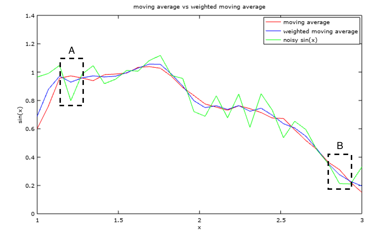
The weight masks generally used are odd sized, as this makes the mask centred around the central pixel. Also, the results are divided by the sum of the weights to scale the results back to one.

The advantage of weighted moving average over normal moving average can be seen in Fig. 5. In region A and B it is clear that while the data (green plot) and weighted moving average (blue plot) are moving in one direction the normal moving average (red plot) is deviating in the other direction. This is usually becuase the normal moving average gives excessive importance to farther off pixels and hence would not catch sudden trend shifts accurately.

Correlation and Cross Correlation Filtering

Filtering in 2D is very similar to the filtering explained in the section above for the 1D filters on noisy signals. The only point of difference lies in the dimensions of the filter kernel i.e. in 2D filtering the filters are 2D. But the octave code for 2D filtering remains the same as shown below using fspecial function.

% function to plot with labels
function plot_with_labels(matrix, color='white')
  size_x = size(matrix, 1);
  size_y = size(matrix, 2);
  imagesc(matrix);
  hold on;
  [X Y] = meshgrid(1:size_x, 1:size_y);
  string = mat2cell(transpose(matrix), ones(size_x, 1), ones(1, size_y));
  text(
    Y(:)-.45,X(:)+.15,
    string,
    'HorizontalAlignment','left', 
    'VerticalAlignment', 'middle',
    'color', color,
    'fontsize', 12);
  grid_x = .5:1:(size_x + .5);
  grid_y = .5:1:(size_y + .5);
  grid1 = [grid_x;grid_y];
  grid2 = repmat([.5;size_x + .5],1,length(grid_x));
  plot(grid1,grid2,'k');
  plot(grid2,grid1,'k');
endfunction

% moving average in 2D
img = zeros(10, 10);
img(3:7, 4:8) = 90;
img(6, 5) = 0;
img(9, 3) = 90;

f_3 = fspecial('average', 3);
f_5 = fspecial('average', 5);

subplot(3, 1, 1);
plot_with_labels(img);
title('original noisy image');

img_3 = imfilter(img, f_3);
subplot(3, 1, 2);
plot_with_labels(img_3);
title('image after average filter with window size 3');

img_5 = imfilter(img, f_5);
subplot(3, 1, 3);
plot_with_labels(img_5);
title('image after average filter with window size 5');

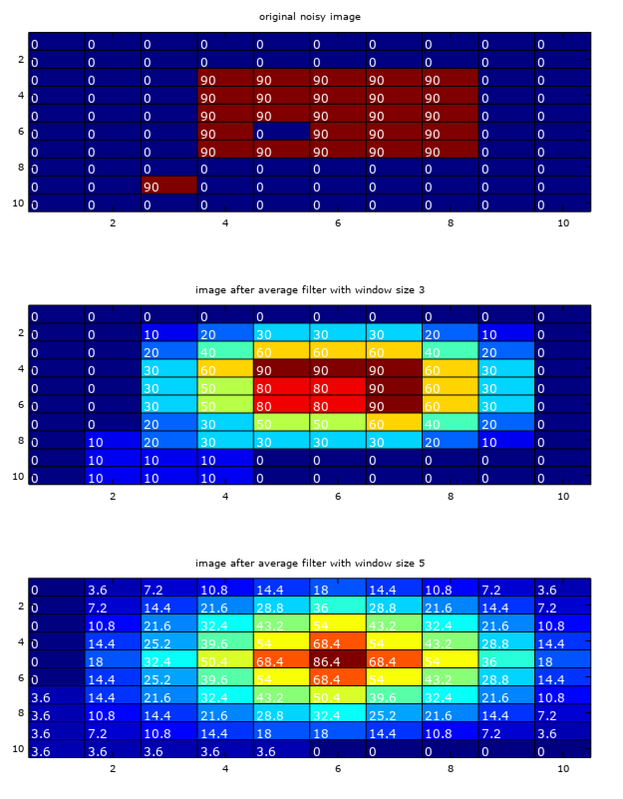
Mathematically, the operation performed in the above code is called correlation filtering with uniform weights. For an averaging window of size \((2k+1 * 2k+1)\) (odd sized window explained in last section), it is given by,

where \(F\) is the image we start with and \(G\) is the final after correlation filtering.

Similarly, one can implement correlation filtering with non-uniform weights, called cross correlation filtering, given by,

where \(G\) is the cross-correlation of \(H\) with \(F\) denoted by

where \(H\) is the matrix of linear weights, also called kernel, mask, or coefficient.

The kernel mentioned here have a slight relation with the machine learning kernels but are entirely different things and hence generally dealt with as seperate topics.

Generally in image processing the average filtering is not used as they are not smooth in magnitude transitions and this is where cross cross-correlation filtering (eg. guassian filter) proves to be advantageuous.

The smoothness of a given filter being applied to an image can be seen from the surface plots and the corresponding effect on the image of a dot as shown below,

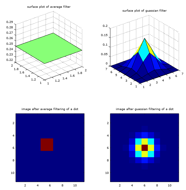
% smoothness of filters
f_average = fspecial('average', 2);
f_smooth = fspecial('gaussian', 7, 1);
img = zeros(11, 11);
img(6,6) = 90;
img_average = imfilter(img, f_average);
img_smooth = imfilter(img, f_smooth);

subplot(2, 2, 1);
surf(f_average);
title('surface plot of average filter');
subplot(2, 2, 2);
surf(f_smooth);
title('surface plot of average filter');
subplot(2, 2, 3);
imagesc(img_average);
title('image after average filtering of a dot');
subplot(2, 2, 4);
imagesc(img_smooth);
title('image after guassian filtering of a dot');

Gaussian Filter

The isotropic (i.e. circularly symmetrical) Guassian function given by,

where sigma is the standard deviation of the function determining the spread of the plot. The effect of \(\sigma\) on the plot can be seen in the plot below.

For more on guassian or normal distribution read Normal Distribution

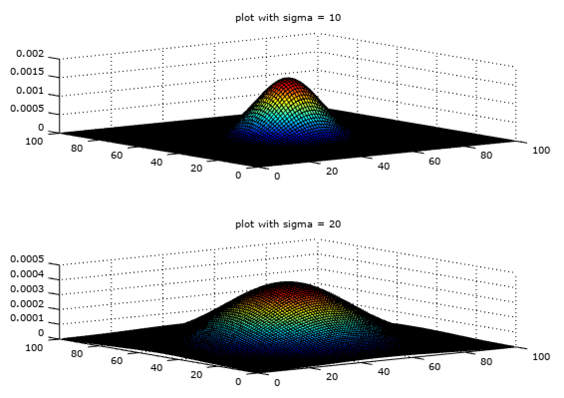
% comparison of sigma
f_gaussian_10 = fspecial('gaussian', 100, 10);
f_gaussian_20 = fspecial('gaussian', 100, 20);
subplot(2, 1, 1);
surf(f_gaussian_10);
title('plot with sigma = 10');
subplot(2, 1, 2);
surf(f_gaussian_20);
title('plot with sigma = 20');

For a given filter size one can vary \(\sigma\) to change the mask or the kernel properties. The bigger the value of \(\sigma\) is the more the blur.

It can be seen from \eqref{7} that the function sigma depends on a single parameter \(\sigma\) that determines the spread of the plot. But, in actual programming, the filter would be represented by a matrix and hence has two properties, namely, size of the matrix and the size of the \(\sigma\).

So one can have different \(\sigma\) within same size of matrix (filter size) as shown in fig 8. The variance (\(\sigma^2\)) or standard deviation (\(\sigma\)) determines the amount of smoothing. The two filters in Fig. 8 have same size but different variance and hence different amount of smoothing.

Similarly, one can have different size matrices (filter size) for the same size of \(\sigma\) (kernel size) as in the plot below.

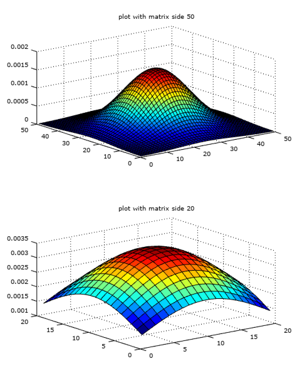
% same sigma in varying size matrix
f_gaussian_50 = fspecial('gaussian', 50, 10);
f_gaussian_20 = fspecial('gaussian', 20, 10);
subplot(2, 1, 1);
surf(f_gaussian_10);
title('plot with matrix side 50');
subplot(2, 1, 2);
surf(f_gaussian_20);
title('plot with matrix side 20');

Among the two, filter of size 50 would work better because it is more smooth among the two.

The Two Sigmas

There are two sigma’s discussed above. One is the intensity of noise and the other is standard deviation of the gaussian filter. The sigma in the intensity of the noise determines the amount of noise added to an image while the sigma of gaussian filter determines the amount of smoothing that occurs on applying the sigma. The two are different that should not be confused.

The reason they are both called sigma is because they both use the normal distribution. The plot of noise signals normal distribution can be seen in Fig. 1 (normal distribution over intensity) and similarly the plot of normal distribution of filtering kernel can be seen in Fig. 9 (isotropic normal distribution in space).

The effect of both the sigmas can be seen in the plot below.

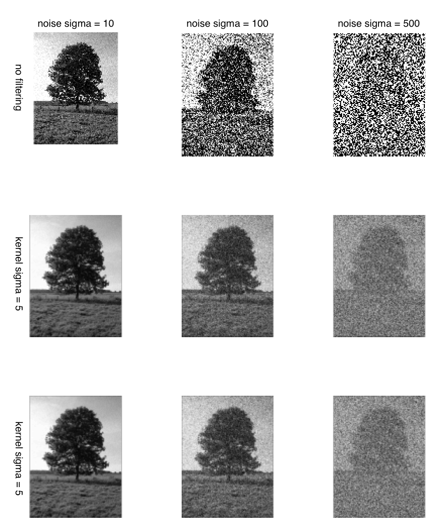
Hence, it is important to understand the difference between the two sigma’s which are generally clear from the context but often create confusion.

REFERENCES:

Introduction to Computer Vision - Udacity