Backpropagation Derivation

The post delves into the mathematics of how backpropagation is defined. It has its roots in partial derivatives and is easily understandable

· · ·

Basics of Machine Learning Series

Index

· · ·

Derivative of Sigmoid

The sigmoid function, represented by $\sigma$ is defined as,

$\sigma(x) = {1 \over 1 + e^{-x}} \tag{1} \label{1}$

So, the derivative of \eqref{1}, denoted by $\sigma’$ can be derived using the quotient rule of differentiation, i.e., if $f$ and $g$ are functions, then,

$\left({f \over g} \right)' = {f'g - g'f \over g^2} \tag{2} \label{2}$

Since $f$ is a constant (i.e. 1) in this case, \eqref{2} reduces to,

$\left({1 \over g} \right)' = {- g' \over g^2} \tag{3} \label{3}$

Also, by the chain rule of differentiation, if $h(x) = f(g(x))$, then,

$h'(x) = f'(g(x)) \cdot g'(x) \tag{4} \label{4}$

Applying \eqref{3} and \eqref{4} to \eqref{1}, $\sigma’(x)$ is given by,

$\begin{align} \sigma'(x) &= -\frac{e^{-x}} {(1+e^{-x})^2} \cdot -1 \\ &= \frac{e^{-x}} {(1+e^{-x})^2} \\ &= {1 \over 1 + e^{-x}} \cdot \frac{1 + e^{-x} - 1} {1+e^{-x}} \\ &= \sigma(x) \cdot \left(\frac{1 + e^{-x}} {1+e^{-x}} - \frac{1} {1+e^{-x}} \right) \\ \sigma'(x) &= \sigma(x) \cdot (1 - \sigma(x)) \tag{5} \label{5} \end{align}$

Mathematics of Backpropagation

(* all the derivations are based scalar calculus and not the matrix calculus for simplicity of calculations)

In most of the cases of algorithms like logistic regression, linear regression, there is no hidden layer, which basically zeroes down to the fact that there is no concept of error propagation in backward direction because there is a direct dependence of model cost function on the single layer of model parameters.

Backpropagation tries to do the similar exercise using the partial derivatives of model output with respect to the individual parameters. It so happens that there is a trend that can be observed when such derivatives are calculated and backpropagation tries to exploit the patterns and hence minimizes the overall computation by reusing the terms already calculated.

Consider a simple neural network with a single path (following the notation from Neural Networks: Cost Function and Backpropagation) as shown below,

Fig-1. Single-Path Neural Network

where,

$\begin{align} a^{(1)} &= x^{(i)} \\ \\ z^{(2)} &= \theta^{(1)} a^{(1)} \\ a^{(2)} &= \sigma(z^{(2)}) \\ \\ z^{(3)} &= \theta^{(2)} a^{(2)} \\ a^{(3)} &= \sigma(z^{(3)}) \\ \\ z^{(4)} &= \theta^{(3)} a^{(3)} \\ a^{(4)} &= g(z^{(4)}) = h(x^{(i)}) = \hat{y}^{(i)} \end{align} \tag{6} \label{6}$

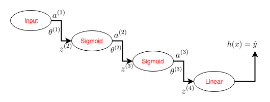
where $g$ is a linear function defined as $g(x) = x$, and hence $g’(x) = 1$. $\sigma$ represents the sigmoid function.

For the simplicity of derivation, let the cost function, $J$ be defined as,

$J = {1 \over 2} (\hat{y}^{(i)} - y^{(i)})^2 \tag{7} \label{7}$

where,

$\delta^{(4)} = \hat{y}^{(i)} - y^{(i)} \tag{8} \label{8}$

Now, in order to find the changes that should be made in the parameters (i.e. weights), partial derivatives of the cost function is calculated w.r.t. individual $\theta’s$,

$\begin{align} \frac {\partial J} {\partial \theta^{(3)}} &= \frac {\partial} {\partial \theta^{(3)}} {1 \over 2} (\hat{y}^{(i)} - y^{(i)})^2 \\ &= (\hat{y}^{(i)} - y^{(i)}) \frac {\partial} {\partial \theta^{(3)}} (g(\theta^{(3)} a^{(3)}) - y^{(i)}) \\ &= (\hat{y}^{(i)} - y^{(i)}) \cdot a^{(3)} \\ &= (\hat{y}^{(i)} - y^{(i)}) \cdot a^{(3)} \tag{9} \label{9} \\ \\ \frac {\partial J} {\partial \theta^{(2)}} &= \frac {\partial} {\partial \theta^{(2)}} {1 \over 2} (\hat{y}^{(i)} - y^{(i)})^2 \\ &= (\hat{y}^{(i)} - y^{(i)}) \frac {\partial} {\partial \theta^{(2)}} (g(\theta^{(3)} \sigma(\theta^{(2)} a^{(2)})) - y^{(i)}) \\ &= (\hat{y}^{(i)} - y^{(i)}) \cdot \theta^{(3)} \sigma'(z^{(3)}) \cdot a^{(2)} \tag{10} \label{10}\\ \\ \frac {\partial J} {\partial \theta^{(1)}} &= \frac {\partial} {\partial \theta^{(1)}} {1 \over 2} (\hat{y}^{(i)} - y^{(i)})^2 \\ &= (\hat{y}^{(i)} - y^{(i)}) \frac {\partial} {\partial \theta^{(1)}} (g(\theta^{(3)} \sigma(\theta^{(2)} \sigma(\theta^{(1)} a^{(1)}))) - y^{(i)}) \\ &= (\hat{y}^{(i)} - y^{(i)}) \cdot \theta^{(3)} \sigma'(z^{(3)}) \cdot \theta^{(2)} \sigma'(z^{(2)}) \cdot a^{(1)} \\ &= (\hat{y}^{(i)} - y^{(i)}) \cdot \theta^{(3)} \sigma'(z^{(3)}) \cdot \theta^{(2)} \sigma'(z^{(2)}) \cdot x^{(i)} \tag{11} \label{11} \end{align}$

One can see a pattern emerging among the partial derivatives of the cost function with respect to the individual parameters matrices. The expressions in \eqref{9}, \eqref{10} and \eqref{11} show that each term consists of the derivative of the network error, the weighted derivative of the node output with respect to the node input leading upto that node.

So, for this network the updates for the matrices are given by,

$\begin{align} \Delta \theta^{(1)} &= - \eta [(\hat{y}^{(i)} - y^{(i)}) \cdot \theta^{(3)} \sigma'(z^{(3)}) \cdot \theta^{(2)} \sigma'(z^{(2)}) \cdot x^{(i)}] \\ \Delta \theta^{(2)} &= - \eta [(\hat{y}^{(i)} - y^{(i)}) \cdot \theta^{(3)} \sigma'(z^{(3)}) \cdot a^{(2)}] \\ \Delta \theta^{(3)} &= - \eta [(\hat{y}^{(i)} - y^{(i)}) \cdot a^{(3)}] \end{align} \tag{12} \label{12}$

Forward propagation is a recursive algorithm takes an input, weighs it along the edges and then applies the activation function in a node and repeats this process until the output node. Similarly, backpropagation is a recursive algorithm performing the inverse of the forward propagation, i.e. it takes the error signal from the output layer, weighs it along the edges and performs derivative of activation in an encountered node until it reaches the input. This brings in the concept of backward error propagation.

Error Signal

Following the concept of backward error propagation, error signal is defined as the accumulated error at each layer. The recursive error signal at a layer l is defined as,

$\delta^{(l)} = \frac {\partial J} {\partial z^{(l)}} \tag{13} \label{13}$

Intuitively, it can be understood as the measure of how the network error changes with respect to the change in input to unit $l$.

So, $\delta^{(4)}$ in \eqref{8}, can be derived using \eqref{13},

$\begin{align} \delta^{(4)} &= \frac {\partial J} {\partial z^{(4)}} = \frac {\partial} {\partial z^{(4)}} {1 \over 2} (\hat{y}^{(i)} - y^{(i)})^2 \\\\ &= (\hat{y}^{(i)} - y^{(i)}) \frac {\partial} {\partial z^{(4)}} (\hat{y}^{(i)} - y^{(i)}) \\ &= (\hat{y}^{(i)} - y^{(i)}) \frac {\partial} {\partial z^{(4)}} (g(z^{(4)}) - y^{(i)}) \\ &= (\hat{y}^{(i)} - y^{(i)}) \tag{14} \label{14} \end{align}$

Similary the error signal at previous layers can be derived and it can be seen how the error signal of the forward layers get transmitted to the backward layers

$\begin{align} \delta^{(3)} &= \frac {\partial J} {\partial z^{(3)}} \\ &= \frac {\partial} {\partial z^{(3)}} {1 \over 2} (\hat{y}^{(i)} - y^{(i)})^2 \\ &= \delta^{(4)} \frac {\partial} {\partial z^{(3)}} (g(\theta^{(3)} \sigma(z^{(3)}))) \\ &= \delta^{(4)} \theta^{(3)} \sigma'(z^{(3)}) \tag{15} \label{15} \\ \\ \delta^{(2)} &= \frac {\partial J} {\partial z^{(2)}} \\ &= \frac {\partial} {\partial z^{(2)}} {1 \over 2} (\hat{y}^{(i)} - y^{(i)})^2 \\ &= \delta^{(4)} \frac {\partial} {\partial z^{(2)}} (g(\theta^{(3)} \sigma(\theta^{(2)} \sigma(z^{(2)})))) \\ &= \delta^{(4)} \theta^{(3)} \sigma'(z^{(3)}) \cdot \theta^{(2)} \sigma'(z^{(2)}) \\ &= \delta^{(3)} \theta^{(2)} \sigma'(z^{(2)}) \tag{16} \label{16} \\ \end{align}$

Using \eqref{14}, \eqref{15} and \eqref{16}, \eqref{12} can be written as,

$\begin{align} \Delta \theta^{(1)} &= - \eta \delta^{(2)} a^{(1)} \\ \Delta \theta^{(2)} &= - \eta \delta^{(3)} a^{(2)} \\ \Delta \theta^{(3)} &= - \eta \delta^{(4)} a^{(3)} \end{align} \tag{17} \label{17}$

which is nothing but the updates to individual parameter matrices based on partial derivatives of cost w.r.t. individual matrices.

Activation Function

Generally, the choice of activation function at the output layer is dependent on the type of cost function. This is mainly to simplify the process of differentiation. For example, as shown in the example above, if the cost function is mean-squared error then choice of linear function as activation for the output layer often helps simplify calculations. Similarly, the cross-entropy loss works well with sigmoid or softmax activation functions. But this is not a hard and fast rule. One is free to use any activation function with any cost function, although the equations for partial derivatives might not look as nice.

Similarly, the choice of activation function in hidden layers are plenty. Although sigmoid functions are widely used, they suffer from vanishing gradient as the depth increases, hence other activations like ReLUs are recommended for deeper neural networks.

REFERENCES:

Artificial Neural Networks: Mathematics of Backpropagation (Part 4)
Which activation function for output layer?

· · ·

Shams S

AIML Resident @ Apple

Backpropagation Derivation

The post delves into the mathematics of how backpropagation is defined. It has its roots in partial derivatives and is easily understandable

Basics of Machine Learning Series

Derivative of Sigmoid

Mathematics of Backpropagation

Error Signal

Activation Function

REFERENCES:

Notes

Recursing the Rabbit Hole