Basics of Machine Learning Series
Backpropagation NumPy Example
import numpy as np

# define XOR training data
X = np.array([
    [0, 0],
    [0, 1],
    [1, 0],
    [1, 1],
])

y = np.atleast_2d([0, 1, 1, 0]).T

print('X.shape:', X.shape)
print('y.shape:', y.shape)

# defining network parameters
# [2, 2, 1] will also work for the XOR problem presented
LAYERS = [2, 2, 2, 1]
ETA = .1
THETA = []

# sigmoid activation function
def sigmoid(x):
    return 1/(1+np.exp(-x))

# derivative of sigmoid activation function
def sigmoid_prime(x):
    return sigmoid(x) * (1-sigmoid(x))

# calculating cost given the prediction and actual vectors
def cost(y_hat, y):
    return np.mean([_ * _ for _ in (y_hat - y)])

# initialing THETA params for all the layers
def initialize_parameters():
    for idx in range(1, len(LAYERS)):
        THETA.append(np.random.rand(LAYERS[idx], LAYERS[idx-1]+1))

# vectorized forward propagation
def forward_propagation(X,initialize=True):
    if initialize:
        initialize_parameters()
    # adding bias column to the input X
    A = [np.hstack((np.ones((X.shape[0],1)), X))]
    Z = []
    activate = False
    for idx, theta in enumerate(THETA):
        Z.append(np.matmul(A[-1], theta.T))
        # adding bias column to the output of previous layer
        A.append(np.hstack((np.ones((Z[-1].shape[0],1)), sigmoid(Z[-1]))))
    # bias is not needed in the final output
    A[-1] = A[-1][:, 1:]
    y_hat = A[-1]
    return A, Z, y_hat

# vectorized backpropagation
def back_propagation(X, y, initialize=True, debug=False, verbose=False):
    # run a forward pass
    A, Z, y_hat = forward_propagation(X, initialize)
    # calculate delta at final output
    del_ = [(y_hat - y) * sigmoid_prime(Z[len(Z)-1])]
    if verbose:
        print(cost(y_hat, y))
    # flag to signify whether a layer has bias column of not
    bias_free = True
    # running in reverse because delta is propagated backwards
    for idx in reversed(range(1, len(THETA))):
        if bias_free:
            # true only for the final layer where there is no bias
            temp = np.matmul(del_[0], THETA[idx]) * np.hstack((np.ones((Z[idx-1].shape[0], 1)), sigmoid_prime(Z[idx-1])))
            bias_free=False
        else:
            # true for all the layers except the input and output layer
            temp = np.matmul(del_[0][:,1:], THETA[idx]) * np.hstack((np.ones((Z[idx-1].shape[0], 1)), sigmoid_prime(Z[idx-1])))
        del_ = [temp] + del_
    del_theta = []
    bias_free = True
    # calculation for the delta in the parameters
    for idx in reversed(range(len(del_))):
        if bias_free:
            # true only for the final layer where there is no bias
            del_theta = [-ETA * np.matmul(del_[idx].T, A[idx])] + del_theta
            bias_free = False
        else:
            # true for all the layers except the input and output layer
            del_theta = [-ETA * np.matmul(del_[idx][:, 1:].T, A[idx])] + del_theta
    # update parameters
    for idx in range(len(THETA)):
        # asserting that the matrix sizes are same
        assert THETA[idx].shape == del_theta[idx].shape
        THETA[idx] = THETA[idx] + del_theta[idx]
    if debug:
        return (A, Z, y_hat, del_, del_theta)

# training epochs
initialize=True
verbose=True
THETA=[]
for i in range(10000):
    if i % 1000 == 0:
        verbose=True
    back_propagation(X, y, initialize, debug=False, verbose=verbose)
    verbose=False
    initialize=False

# inference after training
A, Z, y_hat = forward_propagation(X, initialize=False)

# final output of the network
print(y_hat)
Sometimes, it can been seen that the network get stuck over a few epochs and then continues to converge quickly. It might be due to the fact that the implementation of neural network above is not the most optimum because of using the mean squared error cost function which is not the recommended for classification purposes because of the issues explained in Classification and Logistic Regression.
Gradient Checking
Often times, it is normal for small bugs to creep in the backpropagtion code. There is a very simple way of checking if the written code is bug free. It is based on calculating the slope of cost function manually by taking marginal steps ahead and behind the point at which the gradient is returned by backpropagation.
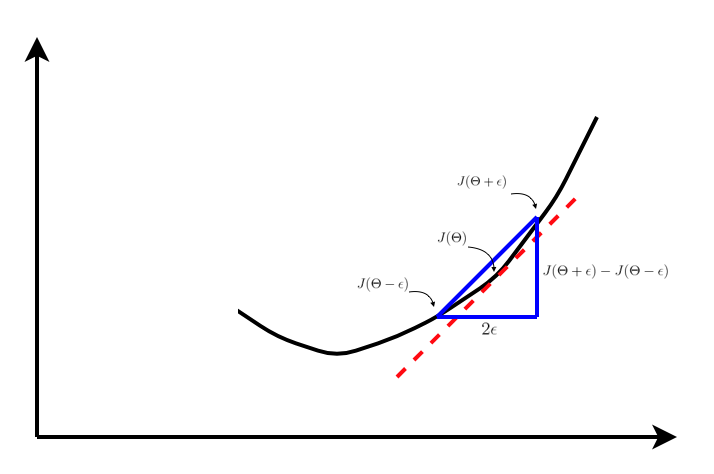
As visible in the plot above, the gradient approximation can be calculated using the centred difference formula as follows,
The approximation in \eqref{1}, works better than the single sided difference, i.e.,
This is basically because if the error is approximated for the terms using Taylor expansion, it is observed that \eqref{1} has error of order \(O(h)\) while \eqref{2} has error of order \(O(h^2)\), i.e. second order approximation.
With multiple parameter matrices, using \eqref{1}, the derivative with respect to \(\Theta_j\) can be approximated as,
Using the NumPy example of backpropagation, gradient checking can be confirmed as follows:
# set epsilon and the index of THETA to check
epsilon = 0.01
idx = 0

# reset THETA and run backpropagation
THETA=[]
A, Z, y_hat, del_, del_theta = back_propagation(X, y, True, True, verbose=True)

# calculate the approximate gradients using centered difference formula
grad_check = np.zeros(THETA[idx].shape)
for i in range(THETA[idx].shape[0]):
    for j in range(THETA[idx].shape[1]):
        THETA[idx][i][j] = THETA[idx][i][j] + epsilon
        A, Z, y_hat = forward_propagation(X, initialize=False)
        J_plus_epsilon = cost(y_hat, y)
        THETA[idx][i][j] = THETA[idx][i][j] - 2* epsilon
        A, Z, y_hat = forward_propagation(X, initialize=False)
        J_minus_epsilon = cost(y_hat, y)
        grad_check[i][j] = (J_plus_epsilon - J_minus_epsilon)/ (2*epsilon)
        THETA[idx][i][j] = THETA[idx][i][j] + epsilon

print("from backprop:")
print(del_theta[idx] / (-2*ETA))
print("from grad check:")
print(grad_check)
Gives output:
from backprop:
[[ 0.00351937  0.00136117  0.00141332]
 [ 0.00254422  0.00088405  0.00082788]]
from grad check:
[[ 0.00353115  0.00136459  0.00141917]
 [ 0.00255167  0.00088687  0.00082796]]
It can be seen that the two values are very similar and hence it proves that the back propagation is working well.
Once the gradient checking is done, it should be turned off before running the network for entire set of training epochs. This is because the numerical approximation of gradient as explained works well for checking the results of backpropagation, but in practice the calculations are much slower than backpropagation and would slow down the training process.
Note: Gradient from backpropagation is adjusted linearly by division with 2. Because of the approximate implementation of backpropagation there is a linear scaling in the derivatives given by the backpropagation function. This still works fine for the overall network because the application of learning rate nullifies the minor scaling error. Let me know if anyone can point out the mistake.
Random Initialization
Initializing all the weights with the same values does not work well because it would basically mean that all the neurons in the following layers will calculate the same functions of the previous layers neurons and hence would have the same updates and would fail to learn anything significant.
Because of this reason, the parameter initialization must be in such a way that it breaks the symmetry and prevents the calculation of similar functions across neurons in the same layer.
Random initialization helps break this symmetry by picking random values between \([-\epsilon, +\epsilon]\)to fill the parameter matrices.
REFERENCES:
Machine Learning: Coursera - Gradient Checking
CS231n Gradient checks