Evaluation of Learning Algorithm

Often it is hard to decide what is right and what is not in evaluating the effectiveness of an algorithm. Which step would should one try and evaluate among the heap of probable options that can help.

· · ·

Basics of Machine Learning Series

Index

· · ·

Problem Statement

It can so happen that, upon applying learning algorithm to a problem statement, there are unacceptably large errors in the predictions made by a model. There are various options that can possibly increase the performance of a model and in turn accuracy, such as,

Acquire more training data
Filter and reduce the number of features
Increase the number of features
Adding polynomial features
Decreasing the regularization parameter, $\lambda$
Increase the regularization parameter, $\lambda$

Seeing the number of options it can often be cumbersome to decide which path should one follow. Because it can so happen that sometimes one or more of the listed techniques might not work in a given case and hence would lead to wasted resources. Hence, randomness and coin toss would not be the correct way of picking one of the options.

Machine Learning Diagnostics are tests that help gain insight about what would or would not work with a learning algorithm, and hence give guidance about how to improve the performance. These can take time to implement, but are still worth venturing into during the time of uncertainties.

Overfitting and Train-Test Split

The case of overfitting in a linear regression is easily detectable by looking at the graph of the plot after determining the parameters as shown in Overfitting and Regularization post. But as the number of features increase it becomes increasingly tough to detect overfitting by plotting.

This is where the standard technique of train-test split comes in handy. It takes care of the scenario where the hypothesis has a low error but still is inaccurate due to overfitting. In this method, given a training dataset, it is split into two sets: training set and test set. Typically, the training set has 70% of the data while test set has the remaining 30%.

The training process is then defined as:

Learn $\Theta$ and minimize $J(\Theta)$ on the training set.
Compute the error, $J_{test}(\Theta)$ on the test set.

Test set error can be defined as follows:

For linear regression, mean-squared error (MSE), defined as,

$J_{test}(\Theta) = {1 \over 2m_{test}} \sum_{i=1}^{m_{test}}(h_{\Theta}(x_{test}^{(i)}) - y_{test}^{(i)})^2 \tag{1} \label{1}$

% vectorized implementation to calculate cost function
error = (X * theta - y);
J = 1 / (2*m) * (error' * error)

Note:Complete Code Sample

For logistic regression, the cross-entropy cost function, defined as,

$J_{test}(\Theta) = {1 \over m_{test}} \sum_{i=1}^{m_{test}} y_{test}^{(i)} log\, h_{\Theta}(x_{test}^{(i)}) + (1 - y_{test}^{(i)}) log\, (1-h_{\Theta}(x_{test}^{(i)})) \tag{2} \label{2}$

Alternative error function, called Misclassification error (0/1 misclassification error) gives the proportion of test data that was misclassified for the logistic regression,

$Test\_Error = {1 \over m_{test}} \sum_{i=1}^{m_{test}} err(h_{\Theta}(x_{test}^{(i)}), y_{test}^{(i)}) \tag{3} \label{3}$

where

$err(h_{\Theta}(x), y) = \begin{cases} 1 \text{, if } h_{\Theta}(x) \geq 0.5 \text{ and } y = 0 \text{ or } h_{\Theta}(x) \lt 0.5 \text{ and } y = 1 \\ 0 \text{, otherwise } \end{cases} \tag{4} \label{4}$

Why Train/Validation/Test Splits?

It is seen that the model error on the training data is generally lower than what error it would display for the unseen data. So it would be fair to say that the loss calculations on the training data are not a proper indicator of the accuracy of the model. For this reason the previous section presented the process of train/test split for checking the performance of the model.

Following the similar argument, say we have $n$ models, having varying candidate hyperparameters (like number of polynomial terms in regression, number of hidden layer and neurons in the neural network) and one is chosen based on the lowest test error it reports after training. Would it be correct to report this error as the indicator of the generalized performance of the selected model?

In general, many practitioners do use the same metrics as model performance, but it is advised against. This is so because, the way the model parameters were fit to the train samples and hence would report lower error on train dataset, similarly the model hyperparameters are fit to the test set and would report a lower error.

To overcome this issue, it is recommended to split the dataset into three parts, namely, train, cross-validation (or validation) and test. Now, train set is used to optimize the model parameters, then cross-validation set is used to select the best model among ones having varying hyperparameters. Finally the generalized performance can be calculated on test dataset which is not seen during training and model selection process. This would be the truly unbiased reporting of model performance metrics. This way the hyperparameters have not been trained using the test set.

Bias vs Variance

Most of the times, if the learning algorithm is not performing well on a dataset, it must be because of a high bias or a high variance problem, which is also sometimes known as underfitting or overfitting problems respectively.

Suppose there is training set for regression split into train, cross validation and test sets. The the training error, $J_{train}(\Theta)$ and cross-validation error, $J_{cv}(\Theta)$ can be defined as follows (based on \eqref{1}),

$J_{train}(\Theta) = {1 \over 2m} \sum_{i=1}^{m}(h_{\Theta}(x^{(i)}) - y^{(i)})^2$ $J_{cv}(\Theta) = {1 \over 2m_{cv}} \sum_{i=1}^{m_{cv}}(h_{\Theta}(x_{cv}^{(i)}) - y_{cv}^{(i)})^2$

As, the degree of regression is increased the learnt parameters would fit the training data better and better and hence reduce the training error. But it would also lead to progressive overfitting after a certain point until when the cross-validation set also performs better, i.e. the error in cross-validation set would decrease initially until the parameters are fit to generalize, but would see a spike in error when the overfitting happens after a certain point. As a result, the plot of degree of regression vs the training and validation error would look as follows.

Fig-1 Bias vs Variance

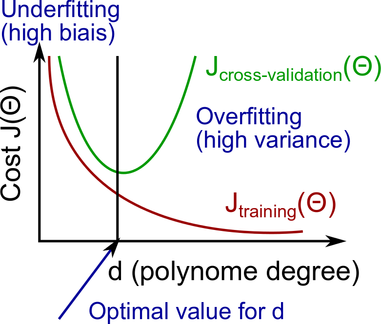
So,

High Bias (Underfitting): both $J_{train}(\Theta)$ and $J_{cv}(\Theta)$ are high and $J_{train}(\Theta) \approx J_{cv}(\Theta)$.
High Variance (Overfitting): $J_{train}(\Theta)$ is low, but $J_{cv}(\Theta)$ is much greater than $J_{train}(\Theta)$.

Effect of Regularization on Bias/Variance

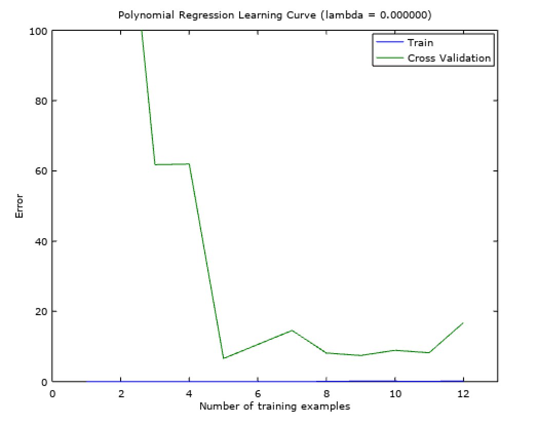
Given a high order polynomial from previous section, if the regularization term, $\lambda$ is small, its equivalent to having a regression without regularization which would have a small train error, $J_{train}(\Theta)$ but would fail to generalize and hence have a high cross-validation error, $J_{cv}(\Theta)$, i.e. a high variance.

Similarly, for a very high value of $\lambda$, since all the parameters would be almost zero, both the training and cross-validation errors would be high, i.e. high bias.

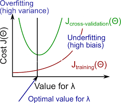
Fig-2 Regularization vs Bias/Variance

Therefore, an optimal value of regularization parameter would balance the tradeoff between the bias-variance and help achieve the ideal model settings.

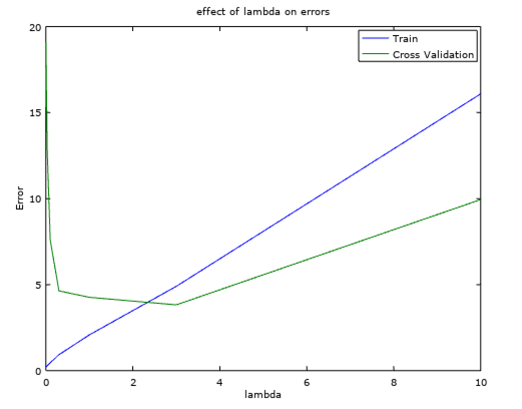
% plot a validation curve that we can use to select lambda
lambda_vec = [0 0.001 0.003 0.01 0.03 0.1 0.3 1 3 10]';

error_train = zeros(length(lambda_vec), 1);
error_val = zeros(length(lambda_vec), 1);

for i = 1:length(lambda_vec)
  lambda = lambda_vec(i);
  [theta] = trainLinearReg(X, y, lambda);
  error_train(i) = linearRegCostFunction(X, y, theta, 0);
  error_val(i) = linearRegCostFunction(Xval, yval, theta, 0);
endfor

Effect of Lambda

Learning Curves

These are the plots of training error and cross-validation errors as a function of number of training data. These plots can give an insight about where the training is suffering from high bias or high variance issues. Fig-3 and Fig-4 show the learning curves for high bias and high variance settings respectively.

Fig-3. High Bias Learning Curves

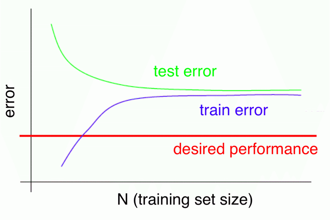
In a high bias setting, as the number of training examples increase the training error would increase too since the model is not fitting the data with an appropriate curve. Also since the generalization is bad, after a certain point, the bias would lead to comparable errors in cross-validation and training. This setting suggests that procuring more data is not going to help improve the model because of the biased assumptions made by the model.

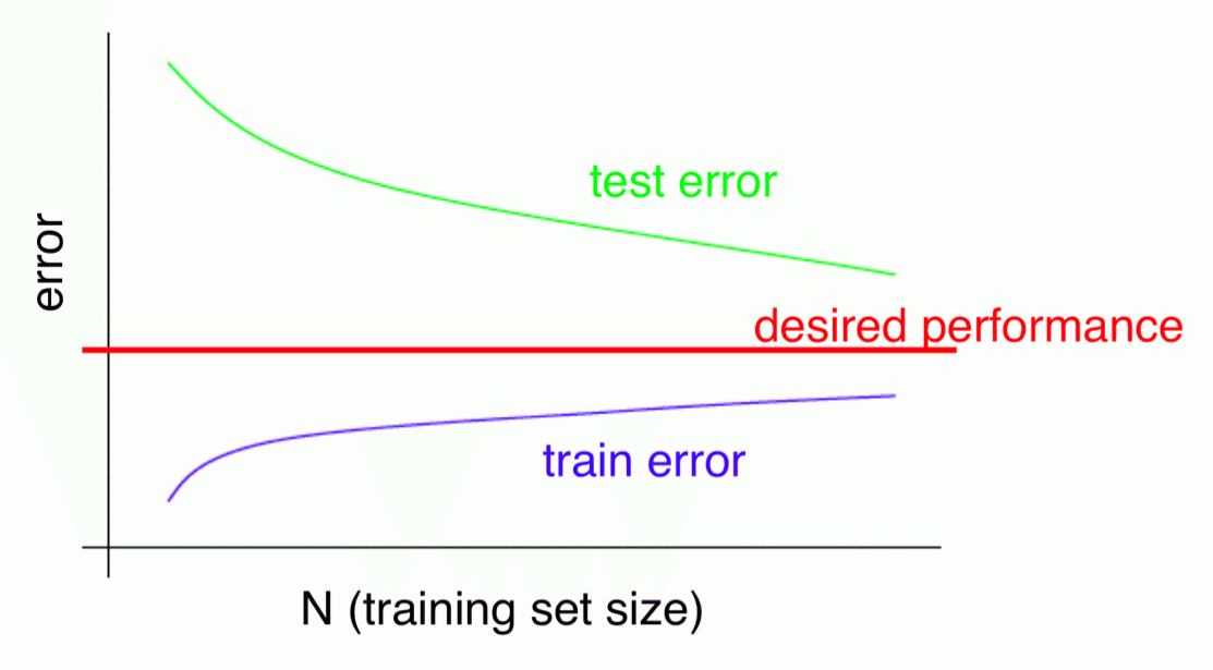
Fig-4. High Variance Learning Curves

In case of high variance, since the order of polynomial is high, the training error will grow slowly but would be well within the desired performance as in the plot above. But the high variance leads to overfitting and hence would cause high cross-validation errors. In this setting, getting more data would help because as the number of training data increases, the model would be forced to learn more generalized parameters that cannot be compensated by a overfit curve. As the plot shows as the number of training data increase, the gap between the training and cross-validation error would close down.

% plot a learning curve
m = size(X, 1);

error_train = zeros(m, 1);
error_val   = zeros(m, 1);

for i = 1: m
  Xi = X(1:i, :);
  yi = y(1:i, :);
  [theta] = trainLinearReg(Xi, yi, lambda);
  error_train(i) = linearRegCostFunction(Xi, yi, theta, 0);
  error_val(i) = linearRegCostFunction(Xval, yval, theta, 0);
endfor

Learning Curves Plot

Summarizing Bias and Variance

So, based on the study of bias and variance, the steps mentions in Problem Statement must be used under following settings:

Acquire more training data fixes high variance
Filtering and reducing the number of features fixes high variance
Increasing the number of features fixes high bias
Adding polynomial features fixes high bias
Decreasing the regularization parameter, $\lambda$, fixes high bias
Increasing the regularization parameter, $\lambda$, fixes high variance

Back to Neural Networks (NN)

NN with less hidden units is prone to underfitting or high bias, but is computationally efficient.
NN with more hidden layers or hidden units is more prone to overfitting or high variance. It is also computationally expensive.

Generally larger nueral networks are used to solve the hard problems of machine learning and the issue of overfitting is solved by choosing and optimal value of regularization parameter, $\lambda$.

Earlier posts suggested using a single hidden layer as the default. Reading this post, it can be seen that one can use the train-validation split to choose the best combination of number of hidden layers.

Recommendations of Experiments

Implement a simple learning algorithm as the first draft to test it on the cross-validation data.
Plot the learning curves to see if there is a high bias or high variance problem and whether increasing training data or working on features is likely to help.
Manual examination of errors can help find the trends in frequent misclassifications.
Error AnalysisGet error results in terms of a single numerical value. Otherwise it would be difficult to assess the performance solely on intuition and would take longer time to analyze. For example, if one uses stemming and sees a rise in accuracy then adding the feature is a definite plus. Hence trying different options and strengthening the process by reinforced numerical estimates will speed up the process of keeping or rejecting features.

The error analysis should be done on cross-validation and not on the test dataset, because test set should be the bearer of actual performance of the model and not used to overfit the features being tested.

REFERENCES:

Machine Learning: Coursera - What to try next?
Machine Learning: Coursera - Evaluating a Hypothesis
Machine Learning: Coursera - Model Selection and Train/Validation/Test Splits
Machine Learning: Coursera - Diagnosing Bias and Variance
Machine Learning: Coursera - Regularization vs Bias Variance
Machine Learning: Coursera - Learning Curves
Machine Learning: Coursera - What to Do Next?

· · ·

Shams S

AIML Resident @ Apple

Evaluation of Learning Algorithm

Often it is hard to decide what is right and what is not in evaluating the effectiveness of an algorithm. Which step would should one try and evaluate among the heap of probable options that can help.

Basics of Machine Learning Series

Problem Statement

Overfitting and Train-Test Split

Why Train/Validation/Test Splits?

Bias vs Variance

Effect of Regularization on Bias/Variance

Learning Curves

Summarizing Bias and Variance

Back to Neural Networks (NN)

Recommendations of Experiments

REFERENCES:

Notes

Recursing the Rabbit Hole