Support Vector Machine

A SVM is a discriminative classifier formally defined by a separating hyperplane. Given labeled training data, the algorithm outputs an optimal hyperplane which categorizes new examples.

· · ·

Basics of Machine Learning Series

Index

· · ·

Optimization Objective

The support vector machine objective can seen as a modification to the cost of logistic regression. Consider the sigmoid function, given as,

$h_\theta(x) = \frac {1} {1 + e^{-z}} \tag{1} \label{1}$

where $z = \theta^T x $

The cost function of logistic regression as in the post Logistic Regression Model, is given by,

$\begin{align} J(\theta) &= -{1 \over m} \sum_{i=1}^m \left( y^{(i)}\,log(h_\theta(x^{(i)}) + (1-y^{(i)})\,log(1 - h_\theta(x^{(i)})) \right) \\ &= -{1 \over m} \sum_{i=1}^m \left( y^{(i)}\,log(\frac {1} {1 + e^{-\theta^T x}}) + (1-y^{(i)})\,log(1 - \frac {1} {1 + e^{-\theta^T x}}) \right) \tag{2} \label{2} \end{align}$

Each training instance contributes to the cost function the following term,

$-y\,log(\frac {1} {1 + e^{-z}}) - (1-y)\,log(1 - \frac {1} {1 + e^{-z}})$

So when $y = 1$, the contributed term is $-log(\frac {1} {1 + e^{-z}})$, which can be seen in the plot below. The cost function of SVM, denoted as $cost_1(z)$, is a modification the former and a close approximation.

Fig-1. SVM Cost function at y = 1

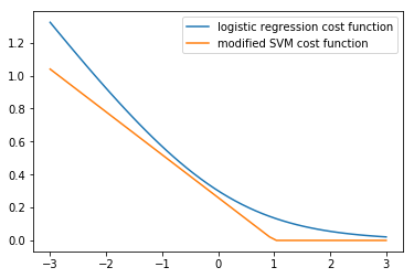
import numpy as np

def svm_cost_1(x):
    return np.array([0 if _ >= 1 else -0.26*(_ - 1) for _ in x])

x = np.linspace(-3, 3)
plt.plot(x, -np.log10(1 / (1+np.exp(np.negative(x)))))
plt.plot(x, svm_cost_1(x))
plt.legend(['logistic regression cost function', 'modified SVM cost function'])
plt.show()

Similarly, when $y = 0$, the contributed term is $-log(1 - \frac {1} {1 + e^{-z}})$, which can be seen in the plot below. The cost function of SVM, denoted as $cost_0(z)$, is a modification the former and a close approximation.

Fig-2. SVM Cost function at y = 0

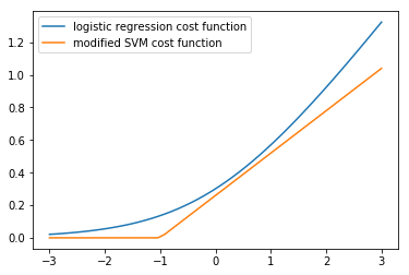
def svm_cost_0(x):
    return np.array([0 if _ <= -1 else 0.26*(_ + 1) for _ in x])

plt.plot(x, -np.log10(1-(1 / (1+np.exp(np.negative(x))))))
plt.plot(x, svm_cost_0(x))
plt.legend(['logistic regression cost function', 'modified SVM cost function'])
plt.show()

While the slope the straight line is not of as much importance, it is the linear approximation that gives SVMs computational advantages that helps in formulating an easier optimization problem.

Regularized version of \eqref{2} can from the post Regularized Logistic Regression can rewritten as,

$J(\theta) = {1 \over m} \sum_{i=1}^m \left( y^{(i)}\,(-log(h_\theta(x^{(i)}))) + (1-y^{(i)})\,(-log(1 - h_\theta(x^{(i)}))) \right) + {\lambda \over 2m } \sum_{j=1}^n \theta_j^2 \tag{3} \label{3}$

In order to come up with the cost function for the SVM, \eqref{3} is modified by replacing the corresponding cost terms, which gives,

$J(\theta) = {1 \over m} \sum_{i=1}^m \left( y^{(i)}\,cost_1(z) + (1-y^{(i)})\,cost_0(z) \right) + {\lambda \over 2m } \sum_{j=1}^n \theta_j^2 \tag{4} \label{4}$

Following the conventions of SVM the following modifications are made to the cost in \eqref{4}, which effectively is a change in notation but not the underlying logic,

removing ${1 \over m}$ does not affect the minimization logic at all as the minima of a function is not changed by the linear scaling.
change the form of parameterization from $A + \lambda B$ to $CA + B$ where it can be intuitively thought that $C = {1 \over \lambda}$.

After applying the above changes, \eqref{4} gives,

$J(\theta) = C \sum_{i=1}^m \left[ y^{(i)}\,cost_1(\theta^T x^{(i)}) + (1-y^{(i)})\,cost_0(\theta^T x^{(i)}) \right] + {1 \over 2 } \sum_{j=1}^n \theta_j^2 \tag{5} \label{5}$

The SVM hypothesis does not predict probability, instead gives hard class labels,

$h_\theta(x) = \begin{cases} 1 \text{, if } \theta^Tx \geq 0 \\ 0 \text{, otherwise} \end{cases} \tag{6} \label{6}$

Large Margin Intuition

Fig-3. SVM Cost function plots

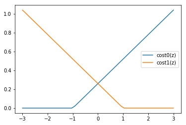
According to \eqref{5} and the plots of the cost function as shown in the image above, the following are two desirable states for SVM,

if $y=1$, then $\theta^Tx \geq 1$ (not just $\geq 0$)
if $y=0$, then $\theta^Tx \leq -1$ (not just $\lt 0$)

Let C in \eqref{5} be a large value. Consequently, in order to minimize the cost, the corresponding term $\sum_{i=1}^m \left[ y^{(i)}\,cost_1(\theta^T x^{(i)}) + (1-y^{(i)})\,cost_0(\theta^T x^{(i)}) \right]$ must be close to 0.

Hence, in order to minimize the cost function, when $y=1$, $cost_1(\theta^T x)$ should be 0, and similarly, when $y=0$, $cost_0(\theta^T x)$ should be 0. And thus, from the plots in Fig.3, it is clear that it can only fulfilled by the two states listed above.

Following the above intuition, the cost function can we written as,

$min_\theta J(\theta) = min_\theta {1 \over 2 } \sum_{j=1}^n \theta_j^2 \tag{7} \label{7}$

subject to contraints,

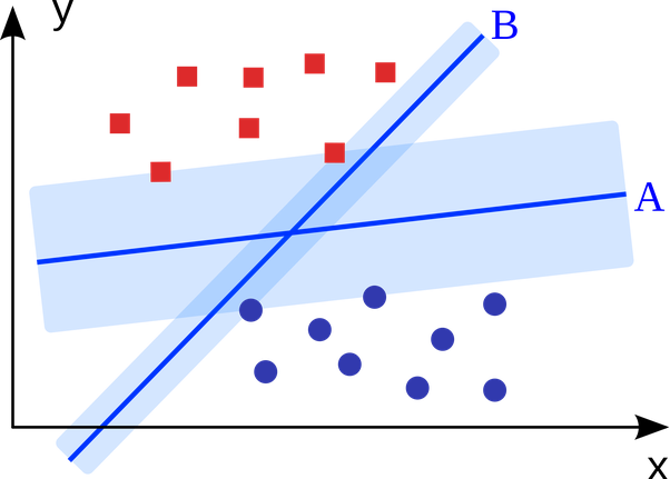
$\begin{align} \theta^Tx^{(i)} &\geq 1 \text{, if } y^{(i)}=1 \\ \theta^Tx^{(i)} &\leq -1 \text{, if } y^{(i)}=0 \end{align}$

What this basically leads to is the selection of a decision boundary that tries to maximize the margin from the support vectors as shown in the plot below. This maximization of the margin as seen for decision boundary A increases the robustness over decision boundaries with lesser margins like B. And it is this property of the SVMs that attributes the name large margin classifier to it.

Fig-4. Large Margin Decision Boundary

Effect of Parameter C

Fig-5. Effect of Parameter C

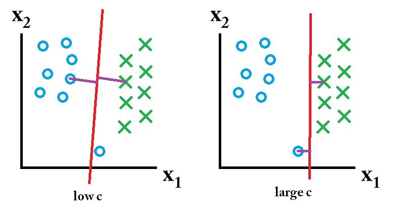
As discussed in the section above, the effect of C can be considered as reciprocal of regularization parameter, $\lambda$. This is more clear from Fig-5. A single outlier, can make the model choose the decision boundary with smaller margin if the value of C is large. A small value of C ensures that the outliers are overlooked and best approximation of large margin boundary is determined.

Mathematical Background

Vector Inner Product: Consider two vectors, $v$ and $w$, given by,

$v = \begin{bmatrix}v_1 \\ v_2 \end{bmatrix}$ $w = \begin{bmatrix}w_1 \\ w_2 \end{bmatrix}$

Then, the inner product or the dot product is defined as $v^Tw = w^Tv$.

Norm of a vector, $v$, denoted as $\lVert v\rVert$ is the euclidean length of the vector given by the pythagoras theorem as,

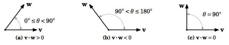
$\lVert v\rVert = \sqrt{\sum_{i=0}^n v_i^2} \in \mathbb{R} \tag{8} \label{8}$

The inner product can also be defined as,

$\begin{align} \text{Inner_Product(v, w)} &= v^Tw = w^Tv = \sum_{i=0}^n v_i \cdot w_i \\ &= \lVert v\rVert \cdot \lVert w\rVert \cdot cos \theta = p \cdot \lVert v\rVert \tag{9} \label{9} \end{align}$

where $p=\lVert w\rVert \cdot cos \theta$ can be described as the projection of vector $w$ onto vector $v$ which can be either positive or negative signed based on the angle $\theta$ between the vectors as shown in the image below.

Fig-6. Dot Product

SVM Decision Boundary: From \eqref{7}, the optimization statement can be written as,

$min_\theta \, {1 \over 2 } \sum_{j=1}^n \theta_j^2 \tag{10} \label{10}$

subject to contraints,

$\begin{align} \theta^Tx^{(i)} &\geq 1 \text{, if } y^{(i)}=1 \\ \theta^Tx^{(i)} &\leq -1 \text{, if } y^{(i)}=0 \end{align} \tag{11} \label{11}$

Let $\theta_0 = 0$ and $n=2$, i.e. number of features is 2 for simplicity, then \eqref{10} can be written as,

$min_\theta \, {1 \over 2 } (\theta_1^2 + \theta_1^2) = {1 \over 2 } \sqrt{(\theta_1^2 + \theta_1^2)}^2 = {1 \over 2 } \lVert \theta \rVert^2 \tag{12} \label{12}$

Using \eqref{9}, $\theta^Tx^{(i)}$ in \eqref{11} can be written as,

$\theta^Tx^{(i)} = p^{(i)} \cdot \lVert \theta \rVert \tag{13} \label{13}$

The plot of \eqref{13} can be seen below,

Fig-7. Dot Product in SVM

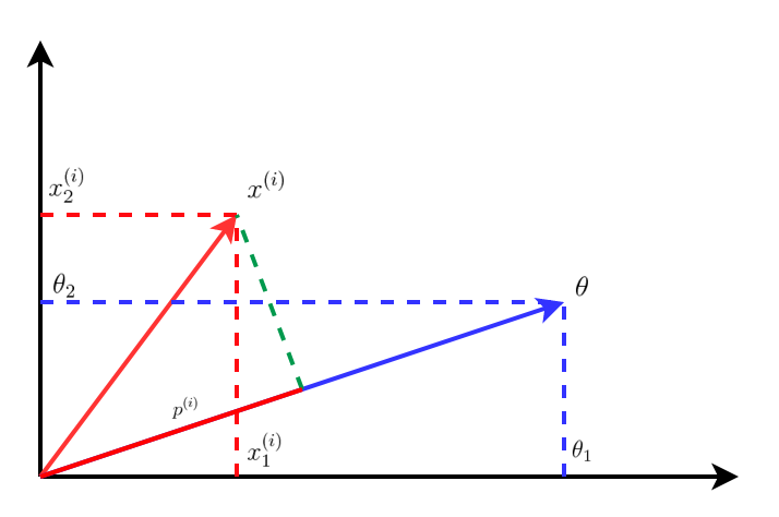
Hence, using \eqref{12} and \eqref{13}, the optimization objective in \eqref{10} and the constraints in \eqref{11} are written as,

$min_\theta \, {1 \over 2 } \lVert \theta \rVert^2 \tag{14} \label{14}$

subject to contraints,

$\begin{align} p^{(i)} \cdot \lVert \theta \rVert &\geq 1 \text{, if } y^{(i)}=1 \\ p^{(i)} \cdot \lVert \theta \rVert &\leq -1 \text{, if } y^{(i)}=0 \end{align} \tag{15} \label{15}$

where $p^{(i)}$ is the projection of $x^{(i)}$ onto vector $\theta$.

Consider two decision boundaries, A and B, and their respective perpendicular parameters, $\theta_A$ and $\theta_B$ as shown in the plot below. As a consequence of choosing $\theta_0 = 0$ for simplification, all the corresponding decision boundaries pass through the origin.

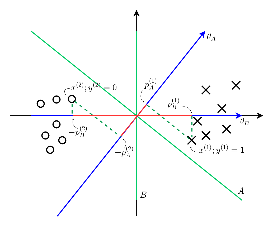
Fig-8. Choosing Large Margin Classifier

Based on the two training examples of either class chosen, close to the boundaries, it can be seen that the magnitude of projection is more in case of $\theta_B$ than $\theta_A$. This basically tells that it would be possible to choose smaller values of $\theta$ and satisfy \eqref{14} and \eqref{15} if the value of projection $p$ is bigger and hence, the decision boundary, B is more favourable to the optimization objective.

Why is decision boundary perpendicular to the $\theta$?

Consider two points $x_1$ and $x_2$ on the decision boundary given by,

$\theta\,x + c= 0 \tag{16} \label{16}$

Since the two points are on the line, they must satisfy \eqref{16}. Substitution leads to the following,

$\theta\,x_1 + c= 0 \tag{17} \label{17}$ $\theta\,x_2 + c= 0 \tag{18} \label{18}$

Subtracting \eqref{18} from \eqref{17},

$\theta\,(x_1 - x_2) = 0 \tag{17} \label{19}$

Since $x_1$ and $x_2$ lie on the line, the vector $(x_1 - x_2)$ is on the line too. Following the property of orthogonal vectors, \eqref{19} is possible only if $\theta$ is orthogonal or perpendicular to $(x_1 - x_2)$, and hence perpendicular to the decision boundary.

Kernels

When dealing with non-linear decision boundaries, a learning method like logistic regression relies on high order polynomial features to find a complex decision boundary and fit the dataset, i.e. predict $y=1$ if,

$\theta_0\,f_0 + \theta_1\,f_1 + \theta_2\,f_2 + \theta_3\,f_3 + \cdots \geq 0 \tag{20} \label{20}$

where $f_0 = x_0,\, f_1=x_1,\, f_2=x_2,\, f_3=x_1x_2,\, f_4=x_1^2,\, \cdots $.

A natural question that arises is if there are choices of better/different features than in \eqref{20}? A SVM does this by picking points in the space called landmarks and defining functions called similarity corresponding to the landmarks.

Fig-9. SVM Landmarks

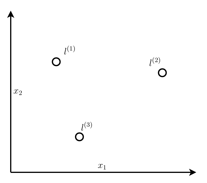
Say, there are three landmarks defined, $l^{(1)}$, $l^{(2)}$ and $l^{(3)}$ as shown in the plot above, the for any given x, $f_1$, $f_2$ and $f_3$ are defined as follows,

$\begin{align} f_1 &= similarity(x, l^{(1)}) = exp \left(- \frac {\lVert x - l^{(1)} \rVert^2} {2 \sigma^2} \right) \\ f_2 &= similarity(x, l^{(2)}) = exp \left(- \frac {\lVert x - l^{(2)} \rVert^2} {2 \sigma^2} \right) \\ f_3 &= similarity(x, l^{(3)}) = exp \left(- \frac {\lVert x - l^{(3)} \rVert^2} {2 \sigma^2} \right) \\ & \vdots \end{align} \tag{21} \label{21}$

Here, the similarity function is mathematically termed a kernel. The specific kernel used in \eqref{21} is called the $Gaussian Kernel$. Kernels are sometimes also denoted as $k(x, l^{(i)})$.

Consider $f_1$ from \eqref{21}. If there exists $x$ close to landmark $l^{(1)}$, then $\lVert x - l^{(1)} \rVert \approx 0$ and hence, $f_1 \approx 1$. Similarly for a $x$ far from the landmark, $\lVert x - l^{(1)} \rVert$ will be a larger value and hence exponential fall will cause $f_1 \approx 0$. So effectively the choice of landmarks has helped in increasing the number of features $x$ had from 2 to 3. which can be helpful in discrimination.

For a gaussian kernel, the value of $\sigma$ defines the spread of the normal distribution. If $\sigma$ is small, the spread will be narrower and when its large the spread will be wider.

Also, the intuition is clear about how landmarks help in generating the new features. Along with the values of parameter, $\theta$ and $\sigma$, various different decision boundaries can be achieved.

How to choose optimal landmarks?

In a complex machine learning problem it would be advantageous to choose a lot more landmarks. This is generally acheived by choosing landmarks at the point of the training examples, i.e. landmarks equal to the number of training examples are chosen, ending up in $l^{(1)}, l^{(2)}, \cdots l^{(m)}$ if there are $m$ training examples. This translates to the fact that each feature is a measure of how close is an instance to the existing points of the class, leading to generation of new feature vectors.

For SVM training, given training examples, $x$, features $f$ are computed, and $y=1$, if $\theta^Tf \geq 0$

The training objective from \eqref{5} is modified as follows,

$min_\theta \, C \sum_{i=1}^m \left[ y^{(i)}\,cost_1(\theta^T f^{(i)}) + (1-y^{(i)})\,cost_0(\theta^T f^{(i)}) \right] + {1 \over 2 } \sum_{j=1}^m \theta_j^2 \tag{22} \label{22}$

In this case, $n=m$ in \eqref{5} by the virtue of procedure used to choose $f$.

The regularization term in \eqref{22} can be written as $\theta^T\theta$. But in practice most SVM libraries, instead $\theta^TM\theta$, which can be considered a scaled version is used as it gives certain optimization benefits and scaling to bigger training sets, which will be taken up at a later point in maybe another post.

While the kernels idea can be applied to other algorithms like logistic regression, the computational tricks that apply to SVMs do not generalize as well to other algorithms.

Hence, SVMs and Kernels tend to go particularly well together.

Bias/Variance

Since $C (= {1 \over \lambda})$,

Large C: Low bias, High Variance
Small C: High bias, Low Variance

Regarding $\sigma$,

Large $\sigma^2$: High Bias, Low Variance (Features vary more smoothly)
Small $\sigma^2$: Low Bias, High Variance (Features vary less smoothly)

Choice of Kernels

Linear Kernel: is equivalent to a no kernel setting giving a standard linear classifier given by,

$\theta_0\,x_0 + \theta_1\,x_1 + \theta_2\,x_2 + \theta_3\,x_3 + \cdots \geq 0 \tag{23} \label{23}$

Linear kernels are used when the number of training data is less but the number of features in the training data is huge.

Gaussian Kernel: Make a choice of $\sigma^2$ to adjust the bias/variance trade-off.

Gaussian kernels are generally used when the number of training data is huge and the number of features are small.

Feature scaling is important when using SVM, especially Gaussian Kernels, because if the ranges vary a lot then the similarity feature would be dominated by features with higher range of values.

All the kernels used for SVM, must satisfy Mercer’s Theorem, to make sure that SVM optimizations do not diverge.

Some other kernels known to be used with SVMs are:

Polynomial kernels, $k(x, l) = (x^T l + constant)^degree$
Esoteric kernels, like string kernel, chi-square kernel, histogram intersection kernel, ..

Multi-Class Classification

Most SVM libraries have multi-class classification.
Alternatively, one may use one-vs-all technique to train $k$ different SVMs and pick class with largest $\theta^Tx$

Logistic Regression vs SVM

If $n$ is large relative to $m$, use logistic regression or SVM with linear kernel, like if $n=10000, m=10-1000$
If $n$ is small and $m$ is intermediate, use SVM with gaussian kernel, like if $n=1-1000, m=10-10000$
If $n$ is small and $m$ is large, create/add more features, then use logistic regression or SVM with no kernel, as with huge datasets SVMs struggle with gaussian kernels, like if $n=1-1000, m=50000+$

Logistic Regression and SVM without a kernel (with linear kernel) generally give very similar. A neural network would work well on these training data too, but would be slower to train.

Also, the optimization problem of SVM is a convex problem, so the issue of getting stuck in local minima is non-existent for SVMs.

REFERENCES:

Machine Learning: Coursera - Optimization Objective
Machine Learning: Coursera - Large Margin Intuition
Machine Learning: Coursera - Mathematics of Large Margin Classification
Machine Learning: Coursera - Kernel I
Machine Learning: Coursera - Kernel II
Machine Learning: Coursera - Using An SVM
Quora - Why is theta perpendicular to the decision boundary?
Introduction to support vector machines

· · ·

Shams S

AIML Resident @ Apple

Support Vector Machine

A SVM is a discriminative classifier formally defined by a separating hyperplane. Given labeled training data, the algorithm outputs an optimal hyperplane which categorizes new examples.

Basics of Machine Learning Series

Optimization Objective

Large Margin Intuition

Effect of Parameter C

Mathematical Background

Kernels

How to choose optimal landmarks?

Bias/Variance

Choice of Kernels

Multi-Class Classification

Logistic Regression vs SVM

REFERENCES:

Notes

Recursing the Rabbit Hole