Principal Component Analysis

A mathematical procedure that transforms a number of (possibly) correlated variables into a (possibly smaller) number of uncorrelated variables called principal components.

· · ·

Basics of Machine Learning Series

Index

· · ·

Introduction

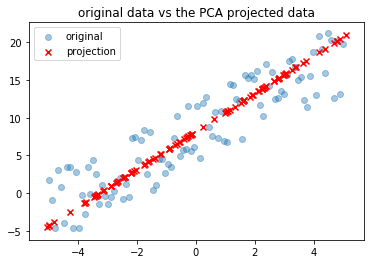
For a given dataset, PCA tries to find a lower dimensional surface onto which these points can be projected while minimizing the approximation losses. For example consider the dataset (marked by blue dots’s) in $\mathbb{R}^2$ in the the plot below. The line formed by the red x’s is the projection of the data from $\mathbb{R}^2$ to $\mathbb{R}$.

Fig-1 PCA Projection

Implementation

Ipython Notebook

# library imports
import matplotlib.pyplot as plt
import numpy as np
from sklearn.decomposition import PCA

# random data generation
X = np.zeros((50, 2))
X[:, 0] = np.linspace(0, 50)
X[:, 1] = X[:, 0]
X = X + 5*np.random.randn(X.shape[0], X.shape[1])

# applying PCA on data
# same number of dimensions will help visualize components
pca = PCA(2)
# reduced number of dimensions will help understand projections
pca_reduce = PCA(1)
# projection on new components found
X_proj = pca_reduce.fit_transform(X)
# rebuilding the data back to original space
X_rebuild = pca_reduce.inverse_transform(X_proj)
X_proj = pca.fit_transform(X)

plt.figure(figsize=(7, 7))

# plot data and projection
plt.scatter(X[:,0], X[:, 1], alpha=0.5, c='green')
plt.scatter(X_rebuild[:, 0], X_rebuild[:, 1], alpha=0.3, c='r')

# plot the components
soa = np.hstack((
    np.ones(pca.components_.shape) * pca.mean_, 
    pca.components_ * np.atleast_2d(
        # components scaled to the length of their variance
        np.sqrt(pca.explained_variance_)
    ).transpose()
))
x, y, u, v = zip(*soa)

ax = plt.gca()
ax.quiver(
    x, y, u, v, 
    angles='xy', 
    scale_units='xy', 
    scale=0.5, 
    color='rb'
)
plt.axis('scaled')
plt.draw()

plt.legend([
    'original', 
    'projection'
])

# plot the projection errors
for p_orig, p_proj in zip(X, X_rebuild):
    plt.plot([p_orig[0], p_proj[0]], [p_orig[1], p_proj[1]], c='g', alpha=0.3)
    
plt.show()

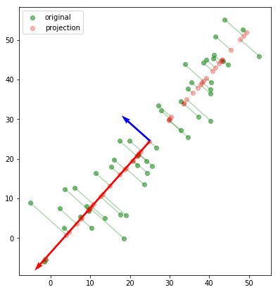
Fig-2 PCA Projection, Components, and Projection Errors

From the above plot it is easier to point out what exactly PCA is doing. The green points show the original data. So all PCA is trying to do is to find the orthogonal components along which the eigenvalues are maximized which is basically a fancy way of saying that PCA finds a feature set in the order of decreasing variance for a given dataset. In the above example, the red vector is displaying higher variance and is the first component, while the blue vector is displaying relatively less variance.

Performing PCA for number of components greater than the current number of dimensions is useless as the data is preserved with 100% variance in the current dimension and no new dimension can help enhance that metric.

So, when dimensionality reduction is done using PCA as can be seen in the red dots, the projection is done along the more dominant feature among the two as it is more representative of the data among the two dimensions. Also, it can be seen that the red vector lies on a line than minimizes the projection losses represented by the green lines from the original data point to the projected data points.

Mean Normalization and feature scaling are a must before performing the PCA, so that the variance of a component is not affected by the disparity in the range of values.

Generalizing to n-dimensional data the same technique can be used to reduce the data to k-dimensions in a similar way by finding the hyper-surface with least projection error.

Projection vs Prediction

PCA is not Linear Regression.

In linear regression, the aim is predict a given dependent variable, $y$ based on independent variables, $x$, i.e. minimize the prediction error. In contrast, PCA does not have a target variable, $y$, it is mere feature reduction by minimizing the projection error. The difference is clear from the plot in Fig-3.

# import the sklearn model
from sklearn.linear_model import LinearRegression

lin_reg = LinearRegression()
lin_reg.fit(X[:,0].reshape(-1, 1), X[:, 1])
# coef_ gives the regression coefficients
y_pred = X[:,0] * lin_reg.coef_

plt.figure(figsize=(7, 7))

# plot data and projection
plt.scatter(X[:,0], X[:, 1], alpha=0.5, c='green')
plt.scatter(X_rebuild[:, 0], X_rebuild[:, 1], alpha=0.3, c='r')
plt.scatter(X[:,0], y_pred, alpha=0.5, c='blue')

# plot the projection errors
for p_orig, p_proj in zip(X, X_rebuild):
    plt.plot([p_orig[0], p_proj[0]], [p_orig[1], p_proj[1]], c='r', alpha=0.3)

# plot the prediction errors
for p_orig, y in zip(X, np.hstack((X[:,0].reshape(-1, 1), y_pred.reshape(-1, 1)))):
    plt.plot([p_orig[0], y[0]], [p_orig[1], y[1]], c='b', alpha=0.3)

Fig-3 Projection vs Prediction

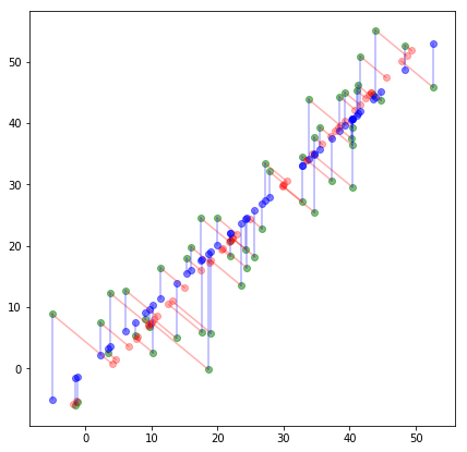
The blue points display the prediction based on linear regression, while the red points display the projection on the reduced dimension. The optimization objectives of the two algorithms are different. While linear regression is trying to minimize the squared errors represented by the blue lines, PCA is trying to minimize the projection errors represented by the red lines.

Mean Normalization and Feature Scaling

It is important to have both these steps in the preprocessing, before PCA is applied. The mean of any feature in a design matrix can be calculated by,

$\mu_j = {1 \over m} \sum_{i=1}^m x_j^{(i)} \label{1} \tag{1}$

Following the calculation of means, the normalization can be done by replacing each $x_j$ by $x_j - \mu_j$. Similarly, feature scaling is done by replacing each $x_j^{(i)}$ by,

$\frac {x_j^{(i)} -\mu_j} {s_j} \label{2} \tag{2}$

where $s_j$ is some measure of the range of values of feature $j$. It can be $max(x_j) - min(x_j)$ or more commonly the standard deviation of the feature.

PCA Algorithm

Compute covariance matrix given by,

$\Sigma = {1 \over m} \sum_{i}^n \left( x^{(i)} \right) \left( x^{(i)} \right)^T \label{3} \tag{3}$

All covariance matrices, $\Sigma$, satisfy a mathematical property called symmetric positive definite. (Will take up in future posts.)

Follow by this, eigen vectors and eigen values are calculated. There are various ways of doing this, most popularly done by singular value decomposition (SVD) of the covariance matrix. SVD returns three different matrices given by,

$U,S,V = SVD(\Sigma) \label{4} \tag{4}$

where,

$\Sigma$ is a $n * n$ matrix because each $x^{(i)}$ is a $n * 1$ vector.
$U$ is the $n * n$ matrix where each column represents a component of the PCA. In order to reduce the dimensionality of the data, one needs to choose the first $k$ columns to form a matrix, $U_{reduce}$, which is a $n * k$ matrix.

So the dimensionally compressed data is given by,

$z^{(i)} = U_{reduce}^T x^{(i)} \label{5} \tag{5}$

Since, $U_{reduce}^T$ is $k * n$ matrix and $x^{(i)}$ is $n * 1$ vector, the product, $z^{(i)}$ is a $k * 1$ vector with reduced number of dimensions.

Given a reduced representation, $z^{(i)}$, we can find its approximate reconstruction in the higher dimension by,

$x_{approx}^{(i)} = U_{reduce} \cdot z^{(i)} \label{6} \tag{6}$

Since, $U_{reduce}$ is $n * k$ matrix and $z^{(i)}$ is $k * 1$ vector, the product, $x_{approx}^{(i)}$ is a $n * 1$ vector with the original number of dimensions.

Number of Principal Components

How to determine the number pricipal components to retain during the dimensionality reduction?

Consider the following two metrics

The objective of PCA is to minimize the projection error given by,

${1 \over m} \sum_{i=1}^m \lVert x^{(i)} - x_{approx}^{(i)} \rVert^2 \label{7} \tag{7}$

Total variation in the data is given by,

${1 \over m} \sum_{i=1}^m \lVert x^{(i)} \rVert^2 \label{8} \tag{8}$

Rule of Thumb is, choose the smallest value of $k$, such that,

$\frac { {1 \over m} \sum_{i=1}^m \lVert x^{(i)} - x_{approx}^{(i)} \rVert^2} { {1 \over m} \sum_{i=1}^m \lVert x^{(i)} \rVert^2} \leq 0.01 (\text{or } 1\%) \label{9} \tag{9}$

i.e. $99\%$ of the variance is retained (Generally values such as $95-90\%$ variance retention are used). It will be seen overtime than often the amount of dimensions reduced is significant while maintaining the 99% variance. (because many features are highly correlated.)

Talking about the amount of variance retained in more informative than citing the number of principal components retained.

So for choosing k the following method could be used,

Try PCA for $k=1$
Compute $U_{reduce}$, $z^{(1)}, z^{(2)}, \cdots, z^{(m)}$, $x_{approx}^{(1)}, x_{approx}^{(2)}, \cdots, x_{approx}^{(m)}$
Check variance retention using \eqref{9}.
Repeat the steps for $k = 2, 3, \cdots$ to satisfy \eqref{9}.

There is an easy work around to bypass this tedious process by using \eqref{4}. The matrix $S$ returned by SVD is a diagonal matrix of eigenvalues corresponding to each of the components in $U$. $S$ is a $n * n$ matrix with diagonal eigenvalues $s_{11}, s_{22}, \cdots, s_{nn}$ and off-diagonal elements equal to 0. Then for a given value of $k$,

$\frac { {1 \over m} \sum_{i=1}^m \lVert x^{(i)} - x_{approx}^{(i)} \rVert^2} { {1 \over m} \sum_{i=1}^m \lVert x^{(i)} \rVert^2} = 1 - \frac {\sum_{i=1}^k s_{ii}} {\sum_{i=1}^n s_{ii}} \label{10} \tag{10}$

Using \eqref{10}, \eqref{9} can be written as,

$\frac {\sum_{i=1}^k s_{ii}} {\sum_{i=1}^n s_{ii}} \gt 0.99 (\text{or } 99\%) \label{11} \tag{11}$

Now, it is easier to calculate the variance retained by iterating over values of $k$ and calculating the value in \eqref{11}.

The value in \eqref{10} is a good metrics to cite as the performance of PCA, as to how well is the reduced dimensional data representing the original data.

Suggestions for Using PCA

Speed up a learning algorithm by reducing the number of features by applying PCA and choosing top-k to maintain 99% variance. PCA should be only applied on the training data to get the $U_{reduce}$ and not on the cross-validation or test data. This is because $U_{reduce}$ is parameter of the model and hence should be only learnt on the training data. Once the matrix is determined, the same mapping can be applied on the other two sets.

Run PCA only on the training data, not on cross-validation or test data.

If using PCA for visualization, it does not make sense to choose $k \gt 3$.
Usage of PCA to reduce overfitting is not correct. The reason it works well in some cases is because it reduces the number of features and hence reduces the variance and increases the bias. But often there are better ways of doing this by using regularization and other similar techniques than use PCA. This would be a bad application of PCA. It is generally adviced against because PCA removes some information without keeping into consideration the target values. While this might work when 99% of the variance is retained, it may as well on various occasions lead to the loss of some useful information. On the other hand, regularization parameters are more optimal for preventing overfitting because while penalizing overfitting they also keep in context the values of the target vector.

Do not use PCA to prevent overfitting. Instead look into regularization.

It is often worth a shot to try any algorithm without using PCA before diving into dimensionality reduction. So, before implementing PCA, implement the models with original dataset. If this does not give desired result, one should move ahead a try using PCA to reduce the number of features. This would also give a worthy baseline score to match the performance of model against once PCA is applied.
PCA can also be used in cases when the original data is too big for the disk space. In such cases, compressed data will give some benefits of space saving by dimensionality reduction.

REFERENCES:

Machine Learning: Coursera - PCA Problem Formulation
Machine Learning: Coursera - Algorithm
Machine Learning: Coursera - Reconstruction
Machine Learning: Coursera - Choosing the number of principal components
Machine Learning: Coursera - Advice

· · ·

Shams S

AIML Resident @ Apple

Principal Component Analysis

A mathematical procedure that transforms a number of (possibly) correlated variables into a (possibly smaller) number of uncorrelated variables called principal components.

Basics of Machine Learning Series

Introduction

Implementation

Projection vs Prediction

Mean Normalization and Feature Scaling

PCA Algorithm

Number of Principal Components

Suggestions for Using PCA

REFERENCES:

Notes

Recursing the Rabbit Hole