Anomaly Detection

In data mining, anomaly detection (also outlier detection) is the identification of items, events or observations which do not conform to an expected pattern or other items in a dataset.

· · ·

Basics of Machine Learning Series

Index

· · ·

Introduction

Anomaly detection is primarily an unsupervised learning problem, but some aspects of it are like supervised learning problems.

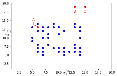
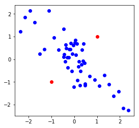
Consider a set of points, $\{x^{(1)}, x^{(2)}, \cdots, x^{(m)}\}$ in a training example (represented by blue points) representing the regular distribution of features $x_1^{(i)}$ and $x_2^{(i)}$. The aim of anomaly detection is to sift out anomalies from the test set (represented by the red points) based on distribution of features in the training example. For example, in the plot below, while point A is not an outlier, point B and C in the test set can be considered to be anomalous (or outliers).

Fig-1 Anomaly

Formally, in anomaly detection the $m$ training examples are considered to be normal or non-anomalous, and then the algorithm must decide if the next example, $x_{test}$ is anomalous or not. So given the training set, it must come up with a model $p(x)$ that gives the probability of a sample being normal (high probability is normal, low probability is anomaly) and resulting decision boundary is defined by,

$\begin{align} p(x_{test}) &\lt \epsilon \text{, flag as outlier or anomaly} \\ p(x_{text}) &\geq \epsilon \text{, flag as normal or non-anomalous} \end{align} \tag{1} \label{1}$

Some of the popular applications of anomaly detection are,

Fraud Detection: A observation set $x^{(i)}$ would represent user $i’s$ activities. Model $p(x)$ is trained on the data from various users and unusual users are identified, by checking which have $p(x^{(i)}) \lt \epsilon $.
Manafacturing: Based on features of products produced on a production line, one can identify the ones with outlier characteristics for quality control and other such preventive measures.
Monitoring Systems in a Data Center: Based on characteristics of a machine behaviour such as CPU load, memory usage etc. it is possible to identify the anomalous machines and prevent failure of nodes in a data-center and initiate diagnostic measures for maximum up-time.

Gaussian Distribution

Gaussian distribution is also called Normal Distribution.

For a basic derivation, refer Normal Distribution.

If $x \in \mathbb{R}$, and $x$ follows Gaussian distribution with mean, $\mu$ and variance $\sigma^2$, denoted as,

$x \sim \mathcal{N}(\mu, \sigma^2) \label{2} \tag{2}$

A standard normal gaussian distribution is a bell-shaped probability distribution curve with mean, $\mu=0$ and standard deviation, $\sigma=1$, as shown in the plot below.

import numpy as np

data = np.random.randn(5000000)
n, x, _ = plt.hist(data, np.linspace(-5, 5, 500))

Fig-2 Gaussian Distribution

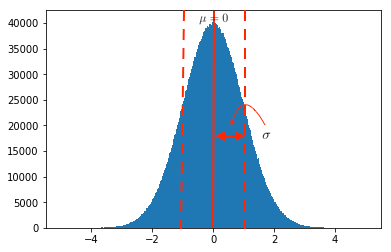
The parameters $\mu$ and $\sigma$ signify the centring and spread of the gaussian curve as marked in the plot above. It can also be seen that the density is higher around the mean and reduces rapidly as distance from mean increases.

The probability of $x$ in a gaussian distribution, $\mathcal{N}(\mu, \sigma^2)$ is given by,

$p(x;\mu, \sigma^2) = {1 \over \sqrt{2\pi} \sigma} exp(- \frac {(x - \mu)^2} {2\sigma^2}) \tag{3} \label{3}$

where,

$\mu$ is the mean,
$\sigma$ is the standard deviation ($\sigma^2$ is the variance)

The effect of mean and standard deviation on a Gaussian plot can be seen clearly in figure below.

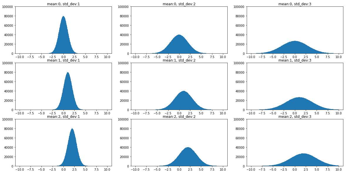
Fig-3 Effect of Mean and Standard Deviation

It can be noticed that, while mean, $\mu$ defines the centering of the distribution, the standard deviation, $\sigma$, defines the spread of the distribution. Also, as the spread increases the height of the plot decreases, because the total area under a probability distribution should always integrate to the value 1.

Given a dataset, as in the previous section, $\{x^{(1)}, x^{(2)}, \cdots, x^{(m)}\}$, it is possible to determine the approximate (or the most fitting) gaussian distribution by using the following parameter estimation,

$\mu = {1 \over m} \sum_{i=1}^m x^{(i)} \tag{4} \label{4}$ $\sigma^2 = {1 \over m} \sum_{i=1}^m (x^{(i)} - \mu)^2 \tag{5} \label{5}$

There is an alternative formula with the constant ${1 \over m-1}$ but in machine learning the formulae \eqref{4} and \eqref{5} are more prevalent. Both are practically very similar for high values of $m$.

Density Estimation Algorithm

The Gaussian distribution explained above, can be used to model an anomaly detection algorithm for a training data, $\{x^{(1)}, x^{(2)}, \cdots, x^{(m)}\}$ where each $x^{(i)}$ is a set of $n$ features, $\{x_2^{(i)}, x_2^{(i)}, \cdots, x_n^{(i)}\}$. Then, $p(x)$ in \eqref{1} is given by,

$p(x) = p(x_1; \mu_1, \sigma_1^2) p(x_2; \mu_2, \sigma_2^2) \cdots p(x_n; \mu_n, \sigma_n^2) \tag{6} \label{6}$

Assumption: The features $\{x_1, x_2, \cdots, x_n\}$ are independent of each other.

where,

$\begin{align} x_1 &\sim \mathcal{N}(\mu_1, \sigma_1^2) \\ x_2 &\sim \mathcal{N}(\mu_2, \sigma_2^2) \\ \vdots \\ x_j &\sim \mathcal{N}(\mu_j, \sigma_j^2) \\ \vdots \\ x_n &\sim \mathcal{N}(\mu_n, \sigma_n^2) \\ \end{align}$

And, \eqref{6}, can be written as,

$p(x) = \prod_{j=1}^n p(x_j; \mu_j, \sigma_j^2) \tag{7} \label{7}$

This estimation of $p(x)$ in \eqref{7} is called the density estimation.

To summarize:

Choose features $x_i$ that are indicative of anomalous behaviour (general properties that define an instance).
Fit parameters, $\mu_1, \cdots, \mu_n, \sigma_1^2, \cdots, \sigma_n^2$, given by,

$\mu_j = {1 \over m} \sum_{i=1}^m x_j^{(i)} \tag{8} \label{8}$ $\sigma_j = {1 \over m} \sum_{i=1}^m (x_j^{(i)} - \mu_j)^2 \tag{9} \label{9}$

Given a new example, compute $p(x)$, using \eqref{6} and \eqref{3}, and mark as anomalous based on \eqref{1}.

Implementation

Ipython Notebook

import matplotlib.pyplot as plt
import numpy as np

X = np.vstack((
    np.random.randint(5, 15, (50, 2)),
    np.random.randint(5, 30, (4, 2)),
))

# split into train and test
X_train = X[:50]
X_test = X[50:]

# density estimation
mu = 1/X_train.shape[0] * np.sum(X_train, axis=0) 
sigma_squared = 1/X_train.shape[0] * np.sum((X_train - mu) ** 2, axis=0)

# probability calculation for test
def p(x, mu, sigma_squared):
    return np.prod(1 / np.sqrt(2*np.pi*sigma_squared) * np.exp(-(x-mu)**2/(2*sigma_squared)), axis=1)

p_test = p(X_test, mu, sigma_squared)

# visualization using contour plot
delta = 0.025
x = np.arange(0, 30, delta)
y = np.arange(0, 30, delta)
x, y = np.meshgrid(x, y)
z = p(np.hstack((x.reshape(-1, 1), y.reshape(-1, 1))), mu, sigma_squared).reshape(x.shape)

plt.figure(figsize=(10, 10))
CS = plt.contour(x, y, z)
plt.clabel(CS, inline=1, fontsize=12)
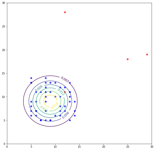
plt.scatter(X[:50, 0], X[:50, 1], c='b', alpha=0.7)
plt.scatter(X[50:, 0], X[50:, 1], c='r', alpha=0.7)

# looking at the plot setting epsilon around p=0.003 seems like a fair value.

Fig-4 Density Estimation

Evaluation of Anomaly Detection System

Single real-valued evaluation metrics would help in considering or rejecting a choice for improvement of an anomaly detection system.

In order to evaluate an anomaly detection system, it is important to have a labeled dataset (similar to a supervised learning algorithm). This dataset would generally be skewed with a high number of normal cases. In order to evaluate the algorithm follow the steps ($y=0$ is normal and $y=1$ is anomalous),

split the examples with $y=0$ into 60-20-20 train-validation-test splits.
split the examples with $y=1$ into 50-50 validation-test splits.
perform density estimation on the train set.
check the performance on the cross-validation set to find out metrics like true positive, true negative, false positive, false negative, precision/recall, f1-score. Accuracy score would not be a valid metric because in most cases the classes would be highly skewed (refer Error Metrics for Skewed Data).
Following this, the value of $\epsilon$ can be altered on the cross-validation set to improved the desired metric in the previous step.
The evalutaion of the final model on the held-out test set would give a unbiased picture of how the model performs.

Anomaly Detection vs Supervised Learning

A natural question arises, “If we have labeled data, why not used a supervised learning algorithm like logistic regression or SVM?”.

Even though there are no hard-and-fast rules about when to use what, there a few recommendations based on observations of learning performance of different algorithms in such settings. They are listed below,

In an anomaly detection setting, it is generally the case that there is a very small number of positive examples (i.e. $y=1$ or the anomalous examples) and a large number of negative examples (i.e. $y=0$ or normal examples). On the contrary, for supervised learning there is a large number of positive and negative examples.
Many a times there are a variety of anomalies that might be presented by a sample (including anomalies that haven’t been presented so far), and if the number of positive set is small to learn from then anomaly detection algorithm stands a better chance in performing better. On the other hand a supervised learning algorithm needs a bigger set of examples from both positive and negative samples to get a sense of the differentiations among the two are as well as the future anomalies are more likely to be the ones presented so far in the training set.

Choosing Features

Feature engineering (or choosing the features which should be used) has a great deal of effect on the performance of an anomaly detection algorithm.

Since the algorithm tries to fit a Gaussian distribution through the dataset, it is always helpful if the the histogram of the data fed to the density estimation looks similar to a Gaussian bell shape.
If the data is not in-line with the shape of a Gaussian bell curve, sometimes a transformation can help bring the feature closer to a Gaussian approximation.

Some of the popular transforms used are,

$log(x)$
$log(x + c)$
$\sqrt{x}$
$x^{ {1 \over 3} }$
Choosing of viable feature options for the algorithm sometimes depends on the domain knowledge as it would help selecting the observations that one is targeting as possible features. For example, network load and requests per minute might a good feature for anomaly detection is a data center. Sometimes it possible to come up with combined features to achieve the same objective. So the rule of thumb is to come up with features that are found to differ substantially among the normal and anomalous examples.

Multivariate Gaussian Distribution

The density estimation seen earlier had the underlying assumption that the features are independent of each other. While the assumption simplifies the analysis there are various downsides to the assumption as well.

Consider the data as shown in the plot below. It can be seen clearly that there is some correlation (negative correlation to be exact) among the two features.

X = np.zeros((50, 2))
X[:10, 0] = np.linspace(0, 20, 10)
X[10:40, 0] = np.linspace(20, 30, 30)
X[40:, 0] = np.linspace(30, 50, 10)
X[:, 1] = -3 * X[:, 0] + 20 * np.random.randn(50,)
X_test = np.array([
    [10., -100.],
    [40., -40.]
])

def normalize(X):
    X_mean = X.mean(axis=0)
    X_std_dev = X.std(axis=0)
    return (X-X_mean)/X_std_dev

X = normalize(X)
X_test = normalize(X_test)

plt.scatter(X[:, 0], X[:, 1], c='b')
plt.scatter(X_test[:, 0], X_test[:, 1], c='r')
plt.axis('scaled')
plt.show()

Fig-5 Correlated Features

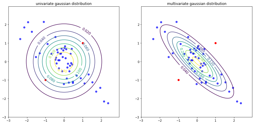
Univariate Gaussian distribution applied to this data results in the following countour plot, which points to the assumption made in \eqref{7}. Because while the two features are negatively correlated, the contour plot do not show any such dependency. On the contrary, if multivariate gaussian distribution is applied to the same data one can point out the correlation. Seeing the difference, it is also clear that the chances of test sets (red points) being marked as normal is lower in multivariate Gaussian than in the other.

mu = X.mean(axis=0)
sigma = X.std(axis=0)
p(X_test, mu, sigma)

mu_mv = 1/X.shape[0] * np.sum(X, axis=0) 
sigma_mv = 1/X.shape[0] * np.matmul((X - mu_mv).transpose(), (X-mu_mv))

def p_mv(x, mu, sigma):
    res = []
    for x_i in x:
        res.append(1 / (2 * np.pi ** (x.shape[1]/2)) / np.sqrt(np.linalg.det(sigma_mv)) *np.exp(-0.5 * np.dot(x_i-mu, np.dot(np.linalg.pinv(sigma), (x_i-mu).transpose()))))
    return np.array(res)

p_mv(X_test, mu_mv, sigma_mv)

plt.figure(figsize=(15, 7))

delta = 0.025
x = np.arange(-3, 3, delta)
y = np.arange(-3, 3, delta)
x, y = np.meshgrid(x, y)
z = p(np.hstack((x.reshape(-1, 1), y.reshape(-1, 1))), mu, sigma_squared).reshape(x.shape)

plt.subplot(1, 2, 1)
CS = plt.contour(x, y, z)
plt.clabel(CS, inline=1, fontsize=12)
plt.scatter(X[:, 0], X[:, 1], c='b', alpha=0.7)
plt.scatter(X_test[:, 0], X_test[:, 1], c='r')
plt.axis('scaled')
plt.title('univariate gaussian distribution')

delta = 0.025
x = np.arange(-3, 3, delta)
y = np.arange(-3, 3, delta)
x, y = np.meshgrid(x, y)
z = p_mv(np.hstack((x.reshape(-1, 1), y.reshape(-1, 1))), mu_mv, sigma_mv).reshape(x.shape)

plt.subplot(1, 2, 2)
CS = plt.contour(x, y, z)
plt.clabel(CS, inline=1, fontsize=12)
plt.scatter(X[:, 0], X[:, 1], c='b', alpha=0.7)
plt.scatter(X_test[:, 0], X_test[:, 1], c='r')
plt.axis('scaled')
plt.title('multivariate gaussian distribution')
plt.show()

Fig-6 Univariate vs Multivariate Gaussian

So, mutlivariate gaussian distribution basically helps model $p(x)$ is one go, unlike \eqref{7}, that models individual features $\{x_1, x_2, \cdots, x_n\}$ in $x$. The multivariate gaussian distribution is given by,

$p(x; \mu, \Sigma) = \frac {1} {(2\pi)^{n/2} \, |\Sigma|^{1/2}} exp\left(-{1 \over 2} (x-\mu)^T \Sigma^{-1} (x-\mu) \right) \tag{10} \label{10}$

where,

$\mu \in \mathbb{R}$ and $\Sigma \in \mathbb{R}^{n * n}$ are the parameters of the distribution.
$|\Sigma|$ is the determinant of the matrix $\Sigma$.

The density estimation for multivariate gaussian distribution can be done using the following 2 formulae,

$\mu = {1 \over m} \sum_{i=1}^m x^{(i)} \tag{11} \label{11}$ $\Sigma = {1 \over m} \sum_{i=1}^m (x^{(i)} - \mu) (x^{(i)} - \mu)^T \tag{12} \label{12}$

Steps in multivariate density estimation:

Given a train dataset, estimate the parameters $\mu$ and $\Sigma$ using \eqref{11} and \eqref{12}.
For a new example $x$, compute $p(x)$ given by \eqref{10}.
Flag as anomaly if $p(x) < \epsilon$.

The covariance matrix is the term that brings in the major difference between the univariate and the multivariate gaussian. The effect of covariance matrix and mean shifting can be seen in the plots below.

A covariance matrix is always symmetric about the main diagonal.

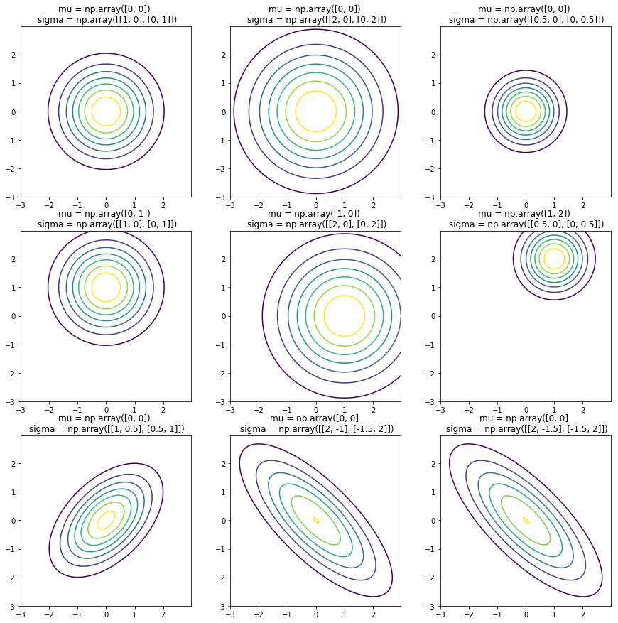
Fig-7 Effect of Mean and Covariance Matrix

The mean shifts the center of the distribution.
Diagonal elements vary the spread of the distribution along corresponding features (also called the variance).
Off-diagonal elements vary the correlation among the various features.

Also, the original model in \eqref{7} is a special case of the multivariate gaussian distribution where the off-diagonal elements of the covariance matrix are contrained to zero (countours are axis aligned).

Univariate vs Multivariate Gaussian Distribution

Univariate model can be used when the features are manually created to capture the anomalies and the features take unusual combinations of values. Whereas multivariate gaussian can be used when the correlation between features is to be captured as well.
Univariate model is computationally cheaper and hence scales well to the larger dataset ($m=10,000-100,000$), whereas the multivariate model is computationally expensive, majorly because of the term $\Sigma_{-1}$.
Univariate model works well for smaller value of $m$ as well. For multivariate model, $m \gt n$, or else $\Sigma$ is singular and hence not invertible.
Generally multivariate gaussian is used when $m$ is much bigger than $n$, like $m \gt 10n$, because $\Sigma$ is a fairly large matrix with around ${n \over 2}$ parameters, which would be learnt better in a setting with larger $m$.

A matrix might be singular because of the presence of redundant features, i.e. two features are linearly dependent or a feature is a linear combination of a set of other features. Such matrices are non-invertible.

REFERENCES:

Machine Learning: Coursera - Problem Motivation
Machine Learning: Coursera - Gaussian Distribution
Machine Learning: Coursera - Algorithm
Machine Learning: Coursera - Anomaly Detection vs Supervised Learning
Machine Learning: Coursera - Multivariate Gaussian Distribution

· · ·

Shams S

AIML Resident @ Apple

Anomaly Detection

In data mining, anomaly detection (also outlier detection) is the identification of items, events or observations which do not conform to an expected pattern or other items in a dataset.

Basics of Machine Learning Series

Introduction

Gaussian Distribution

Density Estimation Algorithm

Evaluation of Anomaly Detection System

Anomaly Detection vs Supervised Learning

Choosing Features

Multivariate Gaussian Distribution

Univariate vs Multivariate Gaussian Distribution

REFERENCES:

Notes

Recursing the Rabbit Hole